10.5.1. Understanding MobileMT Data

In order to properly interpret MobileMT data, it is import to first understand the shape and characteristics of the anomalies due to basic structures. Here, we investigate the MobileMT anomalies by simulating data over a compact conductor. We compare anomalies in MobileMT data to those in classic MT data. And we investigate the impact of the electric fields measured at the base station on MobileMT data.

10.5.1.1. Admittance tensor and MobileMT data

MobileMT systems measure 2 orthogonal horizontal components of the electric field (Ex, Ey) at a base station located on the Earth’s surface, and 3-component magnetic field data (Hx, Hy, Hz) at locations throughout the survey region. For each datum, the components of the magnetic field are linearly related to the measured electric field components at the base station via an admittance tensor \(\mathbf{Y}\), such that:

(1)\[\begin{split}\begin{bmatrix} H_x \\ H_y \\ H_z \end{bmatrix} = \begin{bmatrix} Y_{xx} & Y_{xy} \\ Y_{yx} & Y_{yy} \\ Y_{zx} & Y_{zy} \end{bmatrix} \begin{bmatrix} E_x \\ E_y \end{bmatrix}\end{split}\]

The datum for MobileMT is an apparent conductivity \(\sigma_a\). In much of the theory presented by Expert Geophysics for their MobileMT system, the apparent conductivity is defined via the determinant of the 3x2 admittance tensor as follows:

\[\sigma_a = \mu \omega \big | det(\mathbf{Y}) \big |\]

The exact mathematical justification for evaluating the determinant of the 3x2 matrix is considered proprietary by Expert Geophysics. However, most practitioners assume that since Hz is much weaker than Hx and Hy in the absence of major 3D effects, the last row of the admittance tensor can be neglected and the determinant reduces to:

\[det(\mathbf{Y}) \approx Y_{xx} Y_{yy} - Y_{xy} Y_{yx}\]

For a 3-dimensional Earth, the reduced admittance tensor can be defined using the ratios of electric and magnetic field components in both the x and y directions for 2 orthogonal plane wave polarizations; one polarization with the electric field along the x axis and one polarization with the electric file along the y axis. We can define the reduced admittance tensor as the inverse of the impedance tensor used to define classic MT data. Therefore:

(2)\[\begin{split}\begin{bmatrix} Y_{xx} & Y_{xy} \\ Y_{yx} & Y_{yy} \end{bmatrix} = \begin{bmatrix} H_{x}^{(1)} & H_{x}^{(2)} \\ H_{y}^{(1)} & H_{y}^{(2)} \end{bmatrix} \begin{bmatrix} E_{x}^{(1)} & E_{x}^{(2)} \\ E_{y}^{(1)} & E_{y}^{(2)} \end{bmatrix}^{-1}\end{split}\]

where 1 and 2 refer to fields associated with plane waves polarized along two perpendicular directions. The apparent conductivity values can therefore be computed according to the reduced admittance tensor if the appropriate electric and magnetic field measurements are obtained.

10.5.1.2. MobileMT data over a conductor and a resistor

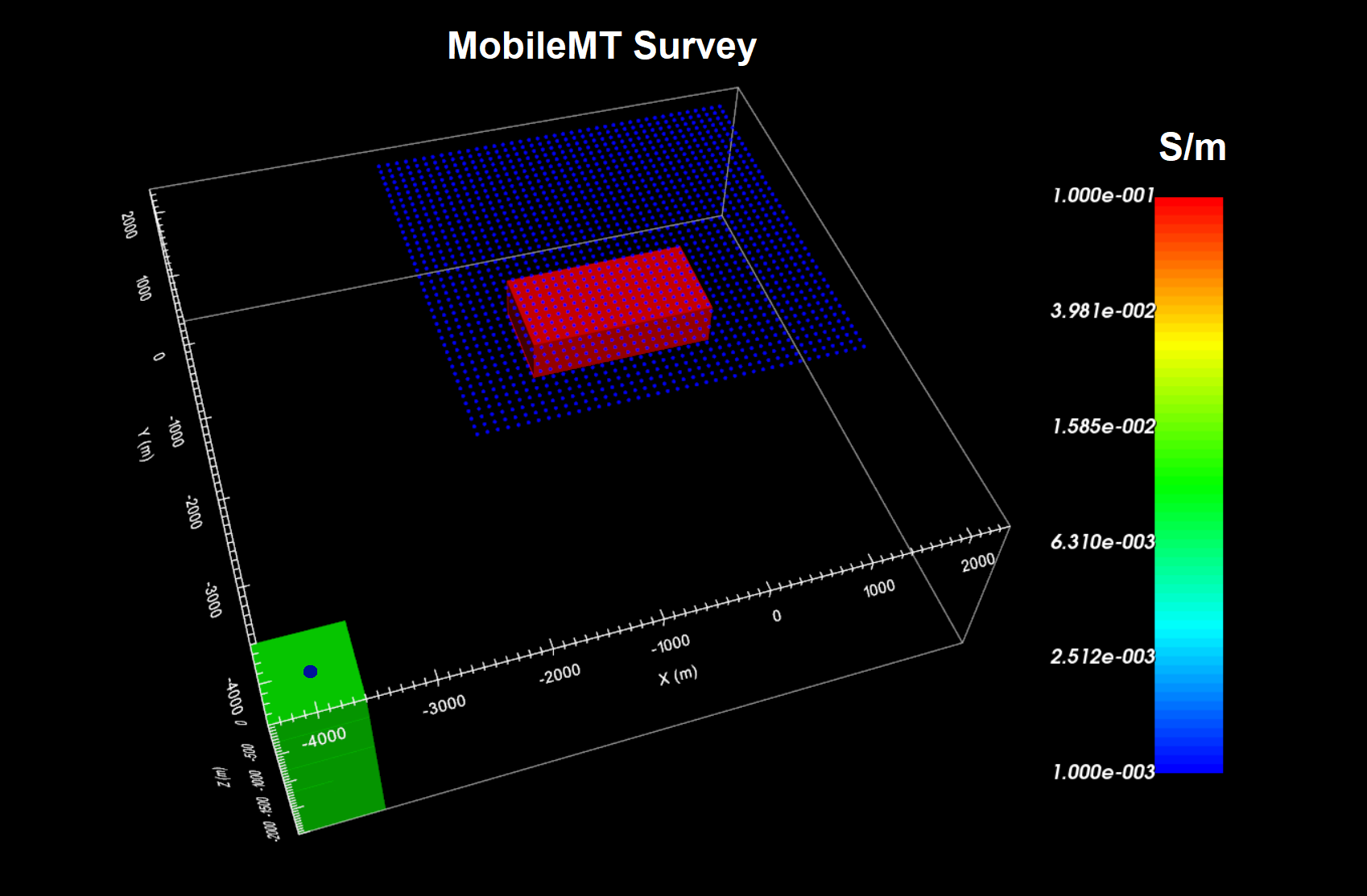
Here, we plot the apparent conductivities from simulated MobileMT data collected over a conductive block and over a resistive block. For each simulation, the block is buried at a depth of 500 m. The East-West dimension of the block is 2000 m and the North-South dimension is 1000 m. The background conductivity is 0.001 S/m. The conductivity of the conductive block is 0.1 S/m. The conductivity of the resistive block is 0.00001 S/m. The base station used to collect horizontal electric field measurements for the MobileMT data is located at (-4000, -4000, 0); far away from the conductor.

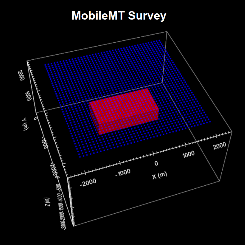
MobileMT survey geometry for a block in a halfspace.

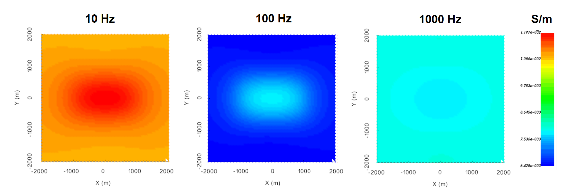
Below, we plot the apparent conductivities at 10 Hz, 100 Hz and 1000 Hz. Away from the block, the apparent conductivities are roughly equal to the background conductivity of 0.001 S/m. This is expected when the background conductivity is homogeneous. For frequencies sensitive to the block, see that the existence of a conductor increases the apparent conductivities, and the existence of a resistor reduces apparent conductivities. At the highest frequency, the skin depth is small and we are not sensitive to the block, so the apparent conductivity more or less equal to the background conductivity.

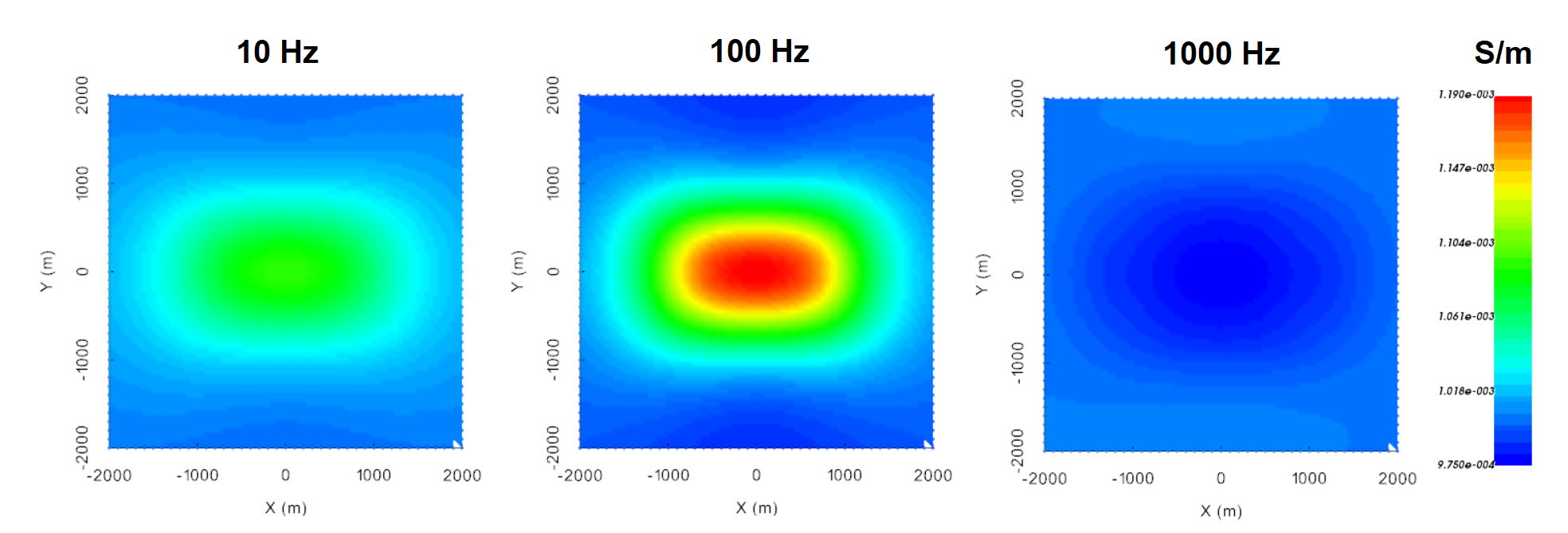
MobileMT apparent conductivities over a conductive block at 10 Hz, 100 Hz and 1000 Hz.

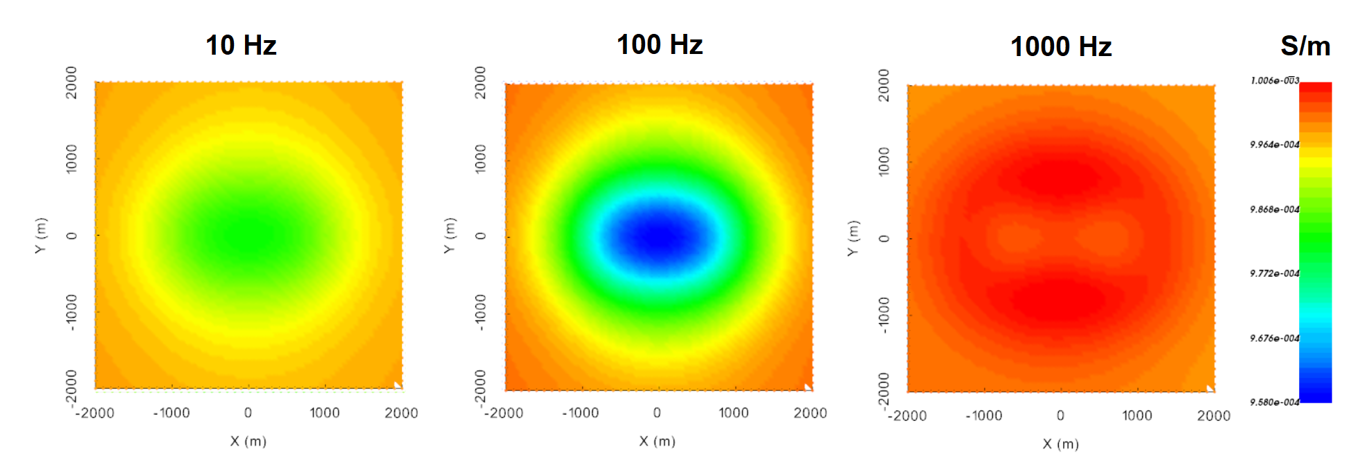
MobileMT apparent conductivities over a resistive block at 10 Hz, 100 Hz and 1000 Hz.

10.5.1.3. MobileMT vs MT data over a compact conductor

Here, the MobileMT data simulated in the previous section is compared to apparent conductivities computed for an MT survey configuration. That is, electric field measurements are now collected throughout the survey region. In this case, the \(Z_{xy}\) impedance is used to compute apparent conductivities from MT data via:

\[\sigma_a = \frac{\omega \mu}{| Z_{xy} |^2}\]

Below, we plot apparent conductivities at 10 Hz, 100 Hz and 1000 Hz. Away from the block, the apparent conductivities in both the MobileMT and classic MT plots are equal to the background conductivity of 0.001 S/m. This is expected when the background conductivity is homogeneous. At the highest frequency, the skin depth is small and we are not sensitive to the block, so the apparent conductivity is once again approximate to the background conductivity.

For both MT and MobileMT, the existence of the conductor reduces the apparent conductivities for frequencies sensitive to the conductor. However, the reduction in apparent conductivity values computed from MT data is much larger than is observed for MobileMT data. And the observed MT anomaly is more compact. This is because MT anomalies are primarily driven by anomalous electric fields throughout the survey region; as anomalous magnetic fields are smoother and lower amplitude. And MobileMT anomalies are driven by anomalous magnetic fields throughout the survey region; as we are now measuring electric fields at a stationary point.

Apparent conductivities from \(Z_{xy}\) impedances at 10 Hz, 100 Hz and 1000 Hz.

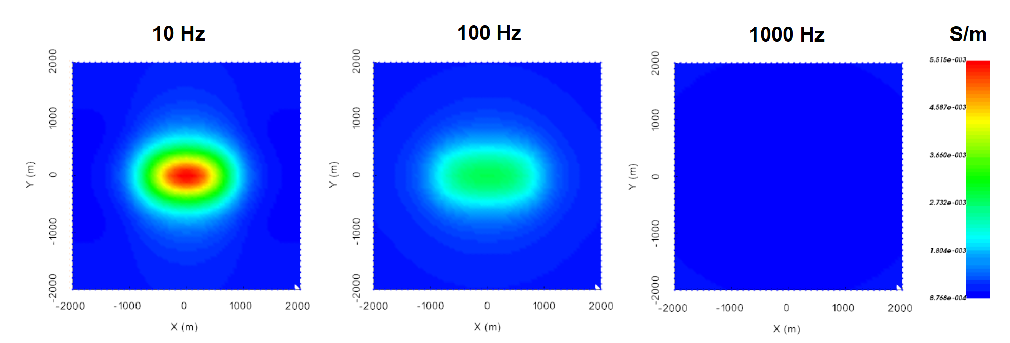
Apparent conductivities from MT data at 10 Hz, 100 Hz and 1000 Hz.

10.5.1.4. Impact of features near the base station

Here, we demonstrate the impact of conductive/resistive structures near the MobileMT base station on the apparent conductivity values. MobileMT data are again simulated over a conductive block. In this case however, the base station (-4000, -4000, 0) is located over a region with a conductivity of 0.01 S/m.

MobileMT survey geometry.

Apparent conductivities are computed using electric field measurements at the base station. Therefore the conductivity near the base station heavily influences MobileMT data. Away from the block, we see that the apparent conductivities are ~0.008 S/m; which is much closer to the base station conductivity than the host conductivity. Essentially, the existence of moderately conductive material at the base station has decreased the amplitude of the measured electric fields, and in turn, increased the magnitudes of all apparent conductivity values. The opposite would be observed if the region around the base station were more resistive. This “shift” in apparent conductivities is observed at other frequencies. However the amplitude of local anomalies relative to the background value for each frequency seem to be relatively well-preserved.

Numerical simulations have shown that the general amplitude of apparent conductivities are primarily driven by the conductivity at the base station. And that anomalies in the MobileMT data result from anomalous magnetic fields due to the presence of conductors and/or resistors within the survey area. So although MobileMT data can be used to infer the existence of anomalous conductors and/or resistors within a region of interest, it may not be suitable for estimating the true conductivity within that region.

MobileMT apparent conductivities for a block in a half-space at 10 Hz, 100 Hz and 1000 Hz.

MobileMT apparent conductivities for a base station conductivity of 0.01 S/m at 10 Hz, 100 Hz and 1000 Hz.