10.8.1. Understanding Borehole UTEM Anomalies

In order to properly interpret borehole UTEM data, it is import to first understand what fields are measured, how the data are plotted and the anomalies for basic structures. Here, we investigate the UTEM anomaly produced by a block in a half-space. The knowledge gained here can be used to determine the coordinate system and sign convention for field collected data, and the operations required to transform the raw data into UBC GIF convention.

10.8.1.1. Introduction to Borehole UTEM

10.8.1.1.1. Survey Geometry and Fundamental Concept

During a borehole UTEM survey, large inductive loop sources are placed on the Earth’s surface. Depending on how each loop is coupled with the target, borehole receivers may be located inside or outside the loop. Data may be collected for several sets of loops and borehole receivers in order to excite the target from multiple directions.

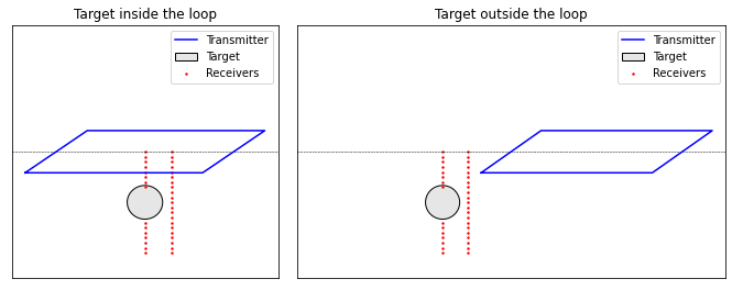
Survey geometry for target near center of the loop (left) and near edge of the loop (right).

During field data collection, standard UTEM systems measure directional components of dB/dt for a highly regulated triangular waveform; see below. However, this is equivalent to measuring the directional components of B(t) for a corresponding step-like waveform. The principal idea of the UTEM system is to collect dB/dt data for the triangular waveform, then transform the raw data so it represents B-field data for the step waveform. The resulting data is effectively the “step response of the Earth”. This is explained in the following subsection.

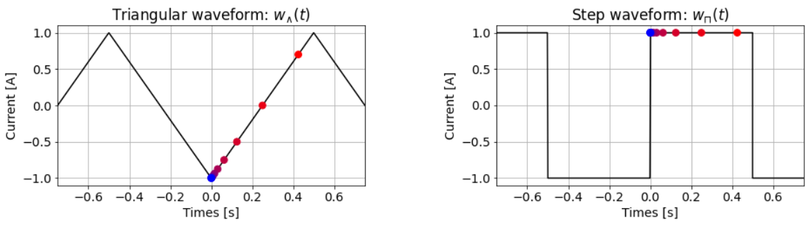
True transmitter waveform and time channels where dB/dt is measured in the field (left). Step waveform and times at which we convert to B-field data (right).

Note

There are modern UTEM systems capable of directly measuring directional components of B(t) for square waveforms.

10.8.1.1.2. Defining UTEM Data

Let \(\xi_b(t)\) represent some impulse response function for the magnetic field observed at a receiver. For the triangular current waveform \(w_{\wedge}(t)\) illustrated above, the B-field at the receiver can be represented as a convolution:

\[B_\wedge (t) = \int_{-\infty}^{\infty} w_\wedge (t) \, \xi_b(t-\tau ) \, d\tau\]

And for the square waveform \(w_{\sqcap}(t)\) illustrated above, the B-field at the receiver can be represented as:

\[B_\sqcap (t) = \int_{-\infty}^{\infty} w_\sqcap (t) \, \xi_b(t-\tau ) \, d\tau\]

By taking the time-derivative of \(w_{\wedge}(t)\), we realize that

\[\frac{d w_{\wedge}}{dt} = \frac{4}{T} w_\sqcap (t)\]

where \(T\) represent the period of both current waveforms. As a result, the time-derivative of the magnetic field observed for the triangular waveform is related to the magnetic field for the step waveform as follows:

\[B_\sqcap (t) = \int_{-\infty}^{\infty} w_\sqcap (t) \, \xi_b(t-\tau ) \, d\tau = \frac{T}{4} \int_{-\infty}^{\infty} \frac{\partial w_\wedge}{\partial t} \, \xi_b(t-\tau ) \, d\tau = \frac{T}{4} \frac{\partial B_\wedge}{\partial t}\]

The above expression shows that raw dB/dt data collected during the survey (normalized by the transmitter current amplitude) can be multiplied by T/4 to obtain equivalent B-field data for the step waveform. And therefore, UTEM data can be defined as 1) the dB/dt response for a triangular waveform, or 2) the B-field for the step waveform. Conventionally, the B-field representation is interpreted to understand the Earth’s response. However, both the dB/dt and B-field representations of the data can be inverted; so long as the correct waveform is used.

10.8.1.1.3. Time Channels

For UTEM systems, the time channels at which the fields are measured depend on the period of the waveform; generally 0.1 s to several seconds. Unlike most TEM systems, the time channels are organized from latest to earliest. Where T denotes the period of the waveform, the time channels for UTEM systems are described below:

• Ch_0: The latest time channel. Data at this time channel is supposed to represent the steady-state B-field expected at a sufficient time after the step-on excitation. Ideally this would be measured at time T/2 , but in practice it is measured slightly earlier.

• Ch_n: These refer to one or two time channels collected at \(t<0\); i.e. before the step-on occurs. For example, we may measure the fields at \(t = -T/2^{13}\) to capture the steady-state B-field the moment before the step excitation.

• Ch_i: Time channels used for interpretation. Most UTEM systems have roughly 10-13 of these time channels. The latest time channel is at time Ch_1 ~ T/4. And from latest to earliest, the time of the channel is decreased by a factor of 2. Thus:

\[Ch \_ i \approx \frac{T}{2^{i+1}}\]

10.8.1.2. Plotting UTEM Data

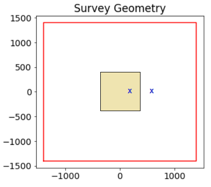
Let us assume the raw field measurements have been converted to the B-field representation for a step waveform with a current amplitude of 1; i.e. \(B_\sqcap (t)\). Here, we define common plotting conventions for UTEM data. The data maps presented here are for UTEM data collected over a conductive block near the middle of a square large loop transmitter. The survey geometry is shown on the right.

Unlike most TEM systems, UTEM instruments measure data during the on-time. The measured fields are dominated by the geometry of the primary field produced by the transmitter. Therefore anomalies resulting from conductive targets are very difficult to identify when the measured fields are plotted directly; see figure below. There are several ways to represent UTEM data that account for the geometry of the transmitter loop and highlight anomalous responses from the Earth. These are defined in the following subsections.

10.8.1.2.1. Normalized by Primary Field

The simplest way to mitigate the masking effect of the primary field is to normalize the data by the absolute value of the primary field. To accomplish this, the path of the transmitter loop must be sufficiently defined by taking GPS coordinates during the survey and converting accordingly to UTM. For each segment of the wire path, the free-space Biot-Savart field can be computed and summed.

Let \(\mathbf{b}_\sqcap(t_i)\) represent the total field at time channel i, and let \(\mathbf{b_p}\) represent the free-space B-field for a current amplitude of 1 A. The data values plotted are given by:

\[\mathbf{d}(t_i) = 100\% \times \Bigg ( \frac{\mathbf{b}_\sqcap(t_i)}{\big | \, \mathbf{b_p} \, \big |} \Bigg )\]

Therefore we are effectively representing the data as a percentage of the primary field.

10.8.1.2.2. Primary Field Reduced Data

For each directional component of the data (e.g. x, y, z), we remove the primary field contribution before normalizing by the magnitude of the primary field. Once again, this requires the path of the transmitter loop be defined by location points collected during the survey.

Where \(\mathbf{b}_\sqcap(t_i)\) represents the total field value at time channel i, and \(\mathbf{b_p}\) represents the free-space magnetic field for a current amplitude of 1 A, the data values plotted are given by:

\[\mathbf{d}(t_i) = 100\% \times \Bigg ( \frac{\mathbf{b}_\sqcap(t_i) - \mathbf{b_p}}{\big | \, \mathbf{b_p} \, \big |} \Bigg )\]

10.8.1.2.3. Channel Reduced Data

For a step excitation, the measured total field should asymptote to the primary field after sufficient time; i.e. when all induced currents have sufficiently diffused. If we assume the inductive response is negligible at the latest time channel (Ch_0), then the data measured at the latest time channel is effectively just the primary field; i.e. \(\mathbf{b}_\sqcap(t_{max}) \approx \mathbf{b_p}\).

The channel reduced representation of the data is given by:

\[\mathbf{d}(t_i) = 100\% \times \Bigg ( \frac{\mathbf{b}_\sqcap(t_i) - \mathbf{b_\sqcap}(t_{max})}{\big | \, \mathbf{b}_\sqcap(t_{max}) \, \big |} \Bigg )\]

The first two plotting approaches depended on having a high level of confidence in the accuracy of the primary field computation. Channel reduced data offers a solution when this is not the case. However, the assumptions we made when defining channel reduced data are not correct in the presence of highly magnetized bodies; i.e. Ch_0 being equivalent to the primary field.

10.8.1.3. Surface UTEM Anomalies

Here, we have chosen to explain the physics in using the B-field resulting from step-excitation (as opposed to the dB/dt representation). We have also chosen to describe anomalies using primary normalized data and NOT primary reduced. For primary reduced data, simply subtract a constant of 100% from any of the data plots.

10.8.1.3.1. Anomaly for a Moderately Conductive Block (Primary Normalized)

Here, we discuss the characteristics of the primary normalized data for a moderately conductive block (1 S/m) within a half-space (0.01 S/m) located near the center of a large square loop. In this case, we assume the period of the waveform is long enough for the secondary fields to decay completely before t = 0 s. Fields are measured several meters above the surface of the Earth. Data maps for the x, y and z components of the B-field normalized by the absolute value of the primary field are plotted below.

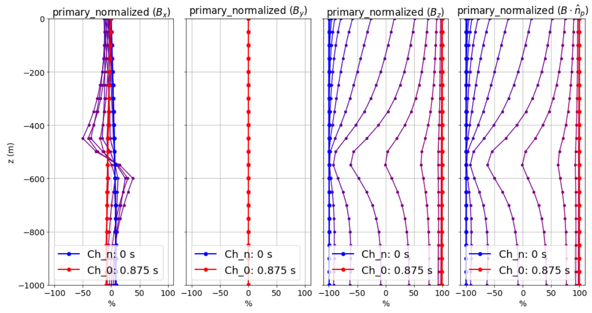
At t = 0:

• We are effectively seeing the steady-state B-field right before the step-on; i.e. the Biot-Savart field for a current of -1 A.

• The primary normalized data projected along the direction of the primary field is -100% everywhere since \(\mathbf{b}_\sqcap (0)=-\mathbf{b_p}\).

At early times:

• At t = 0 s, the primary field changes from \(-\mathbf{b_p}\) to \(\mathbf{b_p}\). This produces a change in magnetic flux density equal to \(2\mathbf{b_p}\)!!!

• Thus at sufficiently early times, currents induced in the ground produce secondary B-fields that are both 1) stronger than and 2) oppose the primary field.

• In the GIF provided, we can actually see the signature of the induced currents as they diffuse away from the transmitter loop over time; especially in the x and y components.

At mid-times:

• Here, “mid-times” refers to time channels where currents induced in the host rock have decayed sufficiently but currents induced in conductive targets have not.

• Over these times, we try to identify conductive targets.

• These time channels are suitable for inversion, as they are sensitive to the target and not the background.

At late-times:

• During the “late-times”, we expect the measured fields to asymptote towards the steady-state B-field long after the step-on; i.e. we expect \(\mathbf{b}_\sqcap (t) \rightarrow \mathbf{b_p}\).

• This occurs at earlier times if the Earth is more resistive and at latter times if the Earth is more conductive; a fact that helps determine the appropriate period for your current waveform.

• The primary normalized data projected along the direction of the primary field should approach 100% everywhere since after sufficient time \(\mathbf{b}_\sqcap (t) \approx \mathbf{b_p}\).

Important

• In the case of primary reduced data, the removal of the free-space primary field effectively shifts the data maps so that they asymptote to 0%. So long as Ch_0 is approximately measuring a steady-state field, this is also true for channel reduced data.

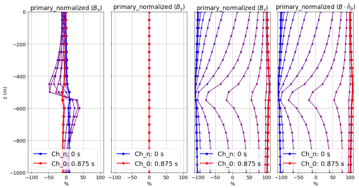
10.8.1.3.2. Anomaly for a Highly Conductive Block (Primary Normalized)

Here, we discuss the characteristics of primary normalized data for a highly conductive block (1000 S/m) in a halfspace (0.01 S/m) located near the center of a large square loop. In this case, the waveform period is not long enough for the induced currents to decay fully over the course of each half-duty cycle. Fields are measured several meters above the surface of the Earth. Data maps for the x, y and z components of the B-field normalized by the absolute value of the primary field are plotted below.

At t = 0:

• Since the induced currents have not fully decayed over the course of the previous half duty cycle (from -T/2 to 0), secondary fields that oppose the primary field are present at t = 0 s.

• Thus the remnants of the signal produced at t < 0 s reduces the amplitude of the primary normalized data.

• This effect can be small (several percent) or very large (as seen above). The more conductive the target, the larger the effect and the more challenging it is to model accurately.

At early times:

• Depending on how conductive the target is (or how short the waveform period is), it may take a number time channels for this signature to dissappear.

At mid-times:

• Unlike in the previous example, it may be more challenging to identify conductive targets at these times.

At late-times:

• At late times, the signal produced by the target has not decayed but is easily distinguishable.

• As t approaches T/2, the primary normalized data plots look like the ones at t = 0 s (except multiplied by -1); i.e. we see the primary normalized data asymptote, just not to 100%.

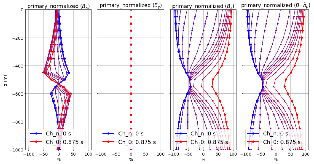
10.8.1.3.3. Anomaly for a Conductive and Susceptible Block (Primary Normalized)

Here, we discuss the characteristics of primary normalized data for a moderately conductive (1 S/m) and magnetically susceptible (1 SI) block in a half-space (0.01 S/m) located near the center of a large square loop. Fields are measured several meters above the surface of the Earth. Data maps for the x, y and z components of the B-field normalized by the absolute value of the primary field are plotted below.

At t = 0:

• We are effectively seeing the steady-state B-field right before the step-on; i.e. for a current of -1 A.

• In this case, the primary normalized data includes the magnetostatic response from the block. Note that primary normalized data projected along the direction of the primary field has anomalous values below -100%.

• The effect of magnetic susceptibility is generally negligible (less than 1%), but can be significant (as seen above) for highly susceptible targets.

At early and mid-times:

• For most rocks, the impact of the magnetic properties on the inductive response is negligible. But for highly susceptible targets (as seen above), the effect is significant.

• In practice, it is better to identify susceptible structures from late time data as opposed to early time data.

• Once again, mid-times can be used to identify conductive targets.

At late-times:

• During the “late-times”, the fields asymptote towards the steady-state for a transmitter current of 1 A; which includes a magnetostatic response.

• It is over these time channels we generally examine the data maps to determine if there are susceptible structures.

• In this case, the primary normalized data projected along the direction of the primary field has values larger than 100% at locations near the susceptible target.