4.8.2.2. Edit Options for Magnetic Inversion Objects
4.8.2.2.1. Mag and Mag Amplitude Inversion (Mag3D)
This functionality is responsible for setting all inversion parameters pertaining to the 3D magnetic inversion codes (Mag inversion and Mag amplitude inversion); see MAG3D background theory. The edit options window is comprised of 3 tabs:
Sensitivity: Sets the mesh, observed data, topography, sensitivity weighting and wavelet compression
Inversion: Sets protocols for the trade-off parameter (\(\beta\)) and all parameters pertaining to the model objective function (alphas, cells weights, upper and lower bounds, active cells, reference models and starting models)
Blocky model norms (ver 5.1 and above): can be activated to recover sparse and blocky models; see sparse and blocky norms
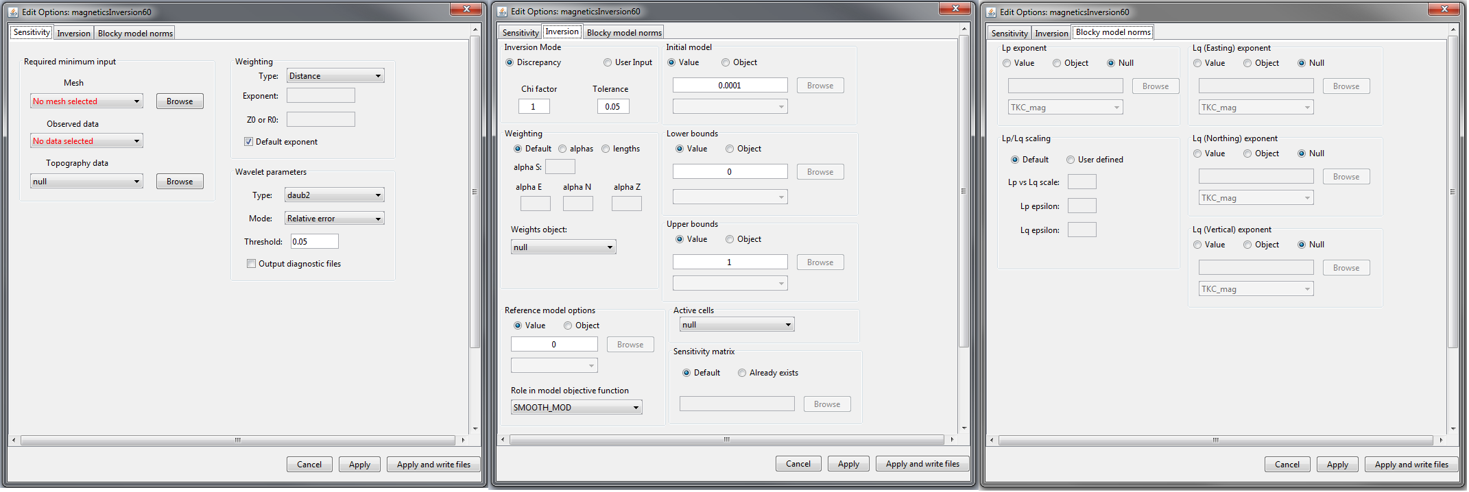
Sensitivity (left), inversion (middle) and blocky model norms (right) tabs for MAG inversion and MAG amplitude inversion objects.
Note
In order to update the set of inversion parameters, you must click apply.
4.8.2.2.1.1. Units
Inputs:
Observed data: total magnetic intensity and amplitude data are given in nanoTeslas (nT)
Reference/background susceptibility model: SI units
Outputs:
Recovered susceptibility model: SI units
4.8.2.2.1.2. Sensitivity Tab
Mesh: mesh for the recovered model
Observed data:
Magnetic data: total magnetic intensity data. Versions 5.0, 5.1 and 6.0
Amplitude data: magnetic amplitude data. Version 6.0 only
Topography: a topography data object. Leave as null for flat topography at an elevation of 0 m.
Weighting: set the type and parameters for sensitivity weighting. The parameters which define the sensitivity weighting are described in the Mag3D manual .
Type: Depth or distance. The choice determines the expression used for the weighting
Exponent: Given by \(\alpha\) in the manual. This parameter has default = 3 to reflect the fact dipolar fields fall of as \(1/r^3\)
Z0 or R0: These constants are defined by equations in the manual. R0 and Z0 are small and generally chosen to be 1/4 the length of the smallest cell dimension
Wavelet parameter: wavelet compression of the sensitivity matrix is used reduced the memory requirements for storing the sensitivity matrix and improve the speed of the inversion algorithm. The details of this are described in the Mag3D manual
Type: sets the type of wavelet transform applied to the rows of the sensitivity matrix
Mode:
Relative error: the level of wavelet compression is specified by a relative threshold (default = 0.05)
Threshold: the level of wavelet compression is specified an absolute threshold
Threshold: user specified value based on choice in mode
4.8.2.2.1.3. Inversion Tab
Inversion Mode: Sets the protocol for the trade-off parameter (\(\beta\) )
Discrepancy: sets the stopping criteria for the inversion using the discrepancy principle. Chi-factor determines the stopping criteria and tolerance sets how close to the ideal stopping criteria before the inversion is terminated.
User Input: the user specifies the exact value for the trade-off parameter (beta )
Weighting: Sets the weights for smallness and smoothness regularization in x, y and z; for relevant equations see manual .
Default: Sets the values of alpha S, alpha X, alpha Y and alpha Z based on cell dimensions
Alphas: Sets specific values for alpha S, alpha X, alpha Y and alpha Z
Lengths: User sets values Len E, Len N and Len Z which define the values of alpha X, alpha Y and alpha Z relative to alpha S. These relationships are given by \(L_x = \sqrt{\frac{\alpha_x}{\alpha_s}}\), \(L_y = \sqrt{\frac{\alpha_y}{\alpha_s}}\) and \(L_z = \sqrt{\frac{\alpha_z}{\alpha_s}}\).
Weighting object: Specify additional cell weights. Use null if no additional model weights are supplied.
Reference model options:
Value: use a constant value to define the reference model
Object: use a GIFmodel as the reference model
Role in objective function: the user selects SMOOTH_MOD or SMOOTH_MOD_DIF. If SMOOTH_MOD is selected, the reference model is included only in the smallness term in the model objective function. If SMOOTH_MOD_DIF is selected, the reference model is included in the smallness and smoothness terms in the model objective function. Further explanation of this is found in fundamentals of inversion.
Initial model:
Value: use a constant value to define a homogeneous starting model
Object: use a GIF model as the starting model
Lower bounds:
Value: set a constant value for the lower bounds for all cells
Object: use a GIF model to supply cell-specific lower bounds
Upper bounds:
Value: set a constant value for the upper bounds for all cells
Object: use a GIF model to supply cell-specific upper bounds
Active cells: Specifies which cells lying below the surface topography are active during the inversion. All other cells remain fixed-valued (equal to starting model). Use null to set all cells lying below surface topography as active.
Sensitivity matrix:
Default: If this option is chosen, the code will generate the sensitivity matrix and save it to the working directory.
Already exists: If the sensitivity matrix for your problem has already been created, this option allows the user to point to the sensitivity file and avoid recomputation
4.8.2.2.1.4. Blocky Model Norms Tab (ver. 5.1 and 6.0)
Sparse and blocky model norms are explained in fundamentals of inversion. Below are parameter descriptions for fields within edit options.
Lp exponent:
Value: set as a constant value \(p \in (0,2]\)
Object: use a GIF model to supply cell-specific values for \(p\)
Null: a default value of \(p=2\) or \(q=2\) is used
Lq exponent (Easting, Northing or Vertical):
Value: set as a constant value \(p \in (0,2]\) or \(q \in (0,2]\)
Object: use a GIF model to supply cell-specific values for \(p\) or \(q\)
Null: a default value of \(p=2\) or \(q=2\) is used
Lp/Lq scaling: the nature of these parameters are discussed in fundamentals of inversion
Lp vs Lq scale: the user alter the weighting between smallness and smoothness while performing the sparse inversion. Default = 1.
Lp epsilon: see fundamentals of inversion
Lq epsilon: see fundamentals of inversion
4.8.2.2.2. MVI Inversion
This functionality is responsible for setting all inversion parameters pertaining to the 3D magnetic vector intensity inversion code. The edit options window is comprised of 4 tabs:
Sensitivity: Sets the mesh, observed data, topography, sensitivity weighting and wavelet compression
Inversion → General: Sets parameters for the magnetic susceptibility model being recovered
Inversion → Vector Options: Sets parameters for the magnetic remanence being recovered
Sparsity: Set the sparsity parameters for the induced and remanent components.
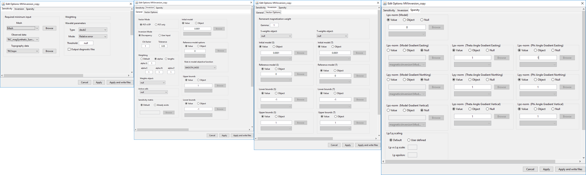
(left) Sensitivity , (middle left) general inversion , (middle right) vector options and (right) sparsity parameter tabs for MVI inversion objects.
Note
In order to update the set of inversion parameters, you must click apply
4.8.2.2.2.1. Units
Inputs:
Observed data: total magnetic intensity data are given in nanoTeslas (nT)
Reference/background susceptibility models for P, S or T: GIF model with effective susceptibility values in SI. Unlike the recovered model, only a single column values is provided.
Norm model: (Mode 2 ATP only): Model norm file for the cell-based sparsity parameter (unitless).
Outputs:
Effective susceptibility model: this model is a 3d vector model containing effective susceptibility values in SI units. The first column contains the effective susceptibility values along the direction of the inducing field. The remaining columns are effective susceptibilities along two orthogonal directions with respect to the inducing field direction.
Angle model: (Mode 2 ATP only) Two models for the vertical (theta) and horizontal (phi) angles in radian.
4.8.2.2.2.2. Sensitivity Tab
Mesh: mesh for the recovered model
Observed data: total magnetic intensity data.
Topography: a topography data object. Leave as null for flat topography at an elevation of 0 m.
Wavelet parameter: wavelet compression of the sensitivity matrix is used reduced the memory requirements for storing the sensitivity matrix and improve the speed of the inversion algorithm. The details of this are described in the Mag3D manual
Type: sets the type of wavelet transform applied to the rows of the sensitivity matrix
- Mode:
Relative error: the level of wavelet compression is specified by a relative threshold (default = 0.05)
Threshold: the level of wavelet compression is specified an absolute threshold
Threshold: (Default null) Search method (recommended), or user specified value based on choice in mode
4.8.2.2.2.3. Inversion (General) Tabs
- Vector Mode: Sets the coordinate system used in the inversion
PST+ATP: First run the smooth inversion in Cartesian coordinate system [PST], followed by an inversion in Spherical system [ATP]. Sparsity only available for this mode.
PST: Only run the smooth inversion in Cartesian coordinates system.
Inversion Mode: Sets the protocol for the trade-off parameter (\(\beta\) )
Discrepancy: sets the stopping criteria for the inversion using the discrepancy principle. Chi-factor determines the stopping criteria and tolerance sets how close to the ideal stopping criteria before the inversion is terminated.
User Input: the user specifies the exact value for the trade-off parameter (beta)
Weighting: Sets the weights for smallness and smoothness regularization in x, y and z; for relevant equations see manual .
Default: Sets the values of alpha S, alpha X, alpha Y and alpha Z based on cell dimensions
Alphas: Sets specific values for alpha S, alpha X, alpha Y and alpha Z
Lengths: User sets values Len E, Len N and Len Z which define the values of alpha X, alpha Y and alpha Z relative to alpha S. These relationships are given by \(L_x = \sqrt{\frac{\alpha_x}{\alpha_s}}\), \(L_y = \sqrt{\frac{\alpha_y}{\alpha_s}}\) and \(L_z = \sqrt{\frac{\alpha_z}{\alpha_s}}\).
Weighting object: Specify additional cell weights. Use null if no additional model weights are supplied.
- Reference model options:
Value: use a constant value to define the reference model
Object: use a GIFmodel as the reference model
Role in objective function: the user selects SMOOTH_MOD or SMOOTH_MOD_DIF. If SMOOTH_MOD is selected, the reference model is included only in the smallness term in the model objective function. If SMOOTH_MOD_DIF is selected, the reference model is included in the smallness and smoothness terms in the model objective function. Further explanation of this is found in fundamentals of inversion.
Initial model:
Value: use a constant value to define a homogeneous starting model for the principle effective susceptibility
Object: use a GIF model as the starting model
Lower bounds:
Value: set a constant value for the lower bounds for all cells
Object: use a GIF model to supply cell-specific lower bounds
Upper bounds:
Value: set a constant value for the upper bounds for all cells
Object: use a GIF model to supply cell-specific upper bounds
Active cells: Specifies which cells lying below the surface topography are active during the inversion. All other cells remain fixed-valued (equal to starting model). Use null to set all cells lying below surface topography as active.
Sensitivity matrix:
Default: If this option is chosen, the code will generate the sensitivity matrix and save it to the working directory.
Already exists: If the sensitivity matrix for your problem has already been created, this option allows the user to point to the sensitivity file and avoid recomputation
4.8.2.2.2.4. Inversion (Vector Options) Tab
Remanent magnetization weight (Gamma): dictates the emphasis at which the inversion explains the data with effective susceptibilities parallel to the inducing field vs orthogonal. Increasing Gamma results in more emphasis being places on magnetization along the inducing field direction (primary component). Defaul = 1.
Initial model (S or T):
Value: use a constant value to define a homogeneous starting model
Object: use a GIF model as the starting model
- Reference model (S or T):
Value: use a constant value to define the reference model
Object: use a GIFmodel as the reference model
Lower bounds (S or T):
Value: set a constant value for the lower bounds for all cells
Object: use a GIF model to supply cell-specific lower bounds
Upper bounds (S or T):
Value: set a constant value for the upper bounds for all cells
Object: use a GIF model to supply cell-specific upper bounds
Weights (S or T): Specify additional cell weights. Use null if no additional model weights are supplied.
4.8.2.2.2.5. Sparsity
- Lps-norm (Model): Norm applied to the vector amplitude either
Value: set a constant value for the approximated norm
Object: use a GIF model to supply cell-specific approximated norm
Null (Default 2)
- Lpx-norm (Model): Norm applied to the gradient of vector amplitude along the x-axis (Easting) either
Value: set a constant value for the approximated norm
Object: use a GIF model to supply cell-specific approximated norm
Null (Default 2)
- Lpy-norm (Model): Norm applied to the gradient of vector amplitude along the y-axis (Northing) either
Value: set a constant value for the approximated norm
Object: use a GIF model to supply cell-specific approximated norm
Null (Default 2)
- Lpz-norm (Model): Norm applied to the gradient of vector amplitude along the z-axis (Vertical) either
Value: set a constant value for the approximated norm
Object: use a GIF model to supply cell-specific approximated norm
Null (Default 2)
- Lpx-norm (Theta): Norm applied to the gradient of Theta angle along the x-axis (Easting) either
Value: set a constant value for the approximated norm
Object: use a GIF model to supply cell-specific approximated norm
Null (Default 2)
- Lpy-norm (Theta): Norm applied to the gradient of Theta angle along the y-axis (Northing) either
Value: set a constant value for the approximated norm
Object: use a GIF model to supply cell-specific approximated norm
Null (Default 2)
- Lpz-norm (Theta): Norm applied to the gradient of Theta angle along the z-axis (Vertical) either
Value: set a constant value for the approximated norm
Object: use a GIF model to supply cell-specific approximated norm
Null (Default 2)
- Lpx-norm (Phi): Norm applied to the gradient of Phi angle along the x-axis (Easting) either
Value: set a constant value for the approximated norm
Object: use a GIF model to supply cell-specific approximated norm
Null (Default 2)
- Lpy-norm (Phi): Norm applied to the gradient of Phi angle along the y-axis (Northing) either
Value: set a constant value for the approximated norm
Object: use a GIF model to supply cell-specific approximated norm
Null (Default 2)
- Lpz-norm (Phi): Norm applied to the gradient of Phi angle along the z-axis (Vertical) either
Value: set a constant value for the approximated norm
Object: use a GIF model to supply cell-specific approximated norm
Null (Default 2)
- Lp/Lp scaling: Master scaling between the model norm and gradient norm
Default: Scale=1, \(epsilon \) found by cooling schedule
- User Defined:
Lp vs Lq scale: Number >0, where 1 = equal penalty
Lp epsilon: Threshold value for model value (effective zero)
Lq epsilon: Threshold value for gradient values (effective zero)