10.4.1. Understanding ZTEM Anomalies

In order to properly interpret Z-axis Tipper electromagnetic (ZTEM) data, it is import to first understand the shape and characteristics of ZTEM anomalies for basic structures. Here, we investigate the ZTEM anomalies produced by compact conductors and resistors. The knowledge gained here can be used to determine the coordinate system and sign convention for field collected data, and the operations required to transform the raw data into UBC GIF convention.

10.4.1.1. ZTEM data definition

During ZTEM surveys, we record the vertical component of the magnetic field (\(H_z\)) everywhere above the survey area while recording the horizontal components (\(H_x\) and \(H_y\) ) at a ground-based reference station. The vertical and horizontal field measurements are related by the following transfer functions:

(1)\[H_z = T_{zx} H_x + T_{zy} H_y\]

For each location, we compute the transfer function values \(T_{zx}\) and \(T_{zy}\), also known as Tippers. For a 3-dimensional Earth, the transfer functions can be defined using the magnetic field components for 2 orthogonal plane-wave polarizations; for example, one polarization with the electric field along the x-axis and one polarization with the electric file along the y-axis. In this case,

(2)\[\begin{split}\begin{bmatrix} H_z^{(1)} \\ H_z^{(2)} \end{bmatrix} = \begin{bmatrix} H_x^{(1)} & H_y^{(1)} \\ H_x^{(2)} & H_y^{(2)} \end{bmatrix} \begin{bmatrix} T_{zx} \\ T_{zy} \end{bmatrix}\end{split}\]

where 1 and 2 refer to fields associated with plane waves polarized along two perpendicular directions. Solving for the transfer functions we obtain:

\[\begin{split}\begin{bmatrix} T_{zx} \\ T_{zy} \end{bmatrix} = \big ( H_x^{(1)} H_y^{(2)} - H_x^{(2)} H_y^{(1)} \big )^{-1} \begin{bmatrix} - H_y^{(1)} H_z^{(2)} + H_y^{(2)} H_z^{(1)} \\ H_x^{(1)} H_z^{(2)} - H_x^{(2)} H_z^{(1)} \end{bmatrix}\end{split}\]

10.4.1.2. ZTEM data and coordinate conventions

ZTEM data are generally defined using a right-handed coordinate system. The question becomes, what direction is x, y and z? And how does this impact the shape of the observed ZTEM anomalies?

UBC-GIF Tipper data are defined in a coordinate system where:

X is Northing

Y is Easting

Z is +ve downward

Most airborne systems define their Tipper data in a coordinate system where:

X is the along-line direction or “flight line direction” (degrees counter-clockwise from Northing)

Y is cross-line direction (90 degrees counter clockwise from along-line direction)

Z is +ve upwards

Below, we see the ZTEM anomalies for UBC-GIF modeled data and standard airborne data collected over the same compact conductor. The standard airborne data were collected along flight lines with a bearing of 45 degrees (from SW to NE). Thus the cross-line direction is -45 degrees (SE to NW). Looking at these anomalies, we see that:

The response near the edges of the conductor is large and the response directly over the conductor is relatively small; as ZTEM measurements are sensitive to lateral changes in conductivity and not the conductor itself.

For UBC-GIF convention, the \(T_{zx}\) anomalies lie to the North and South of the conductor and \(T_{zy}\) anomalies lie to the East and West.

For standard airborne data, the \(T_{zx}\) anomalies are oriented along the flight-direction (along-line) and \(T_{zy}\) anomalies are oriented in the cross-line direction.

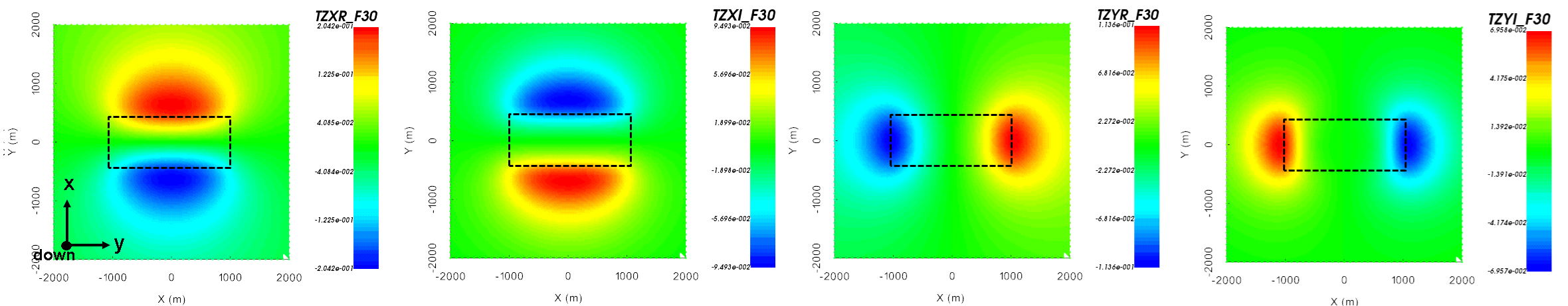
../../../_images/conductor_anomaly_ubcgif.png — ZTEM anomaly in UBC-GIF coordinates over a compact conductor at 30 Hz. From left to right: Re[Tzx], Im[Tzx], Re[Tzy] and Im[Tzy].

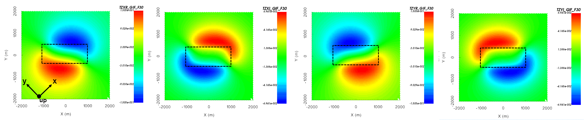
../../../_images/conductor_anomaly_airborne_45.png — ZTEM anomaly in airborne data coordinate system at 30 Hz. Flight lines were at 45 degree (SW to NE) From left to right: Re[Tzx], Im[Tzx], Re[Tzy] and Im[Tzy].

Note

The process of transforming data from the field coordinate system to UBC-GIF is discussed further down on the page.

10.4.1.3. Anomaly over a compact conductor

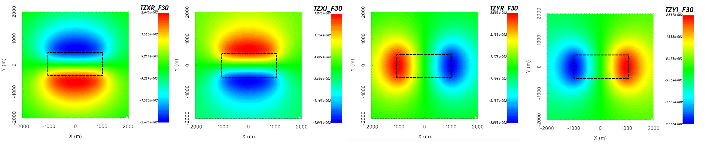
Let us work in the UBC-GIF ZTEM data convention; where X is Northing, Y is Easting and Z is +ve downward. The real and imaginary components of the \(T_{zx}\) and \(T_{zy}\) anomalies over a conductive block are shown below. The conductor is buried at a depth of 200 m. Its East-West dimension is 2000 m and its North-South dimension is 1000 m. The background conductivity is 0.001 S/m and the conductivity of the block is 0.1 S/m. We can see that:

The response near the edges of the conductor is large and the response directly over the conductor is relatively small; as ZTEM measurements are sensitive to lateral changes in conductivity and not the conductor itself.

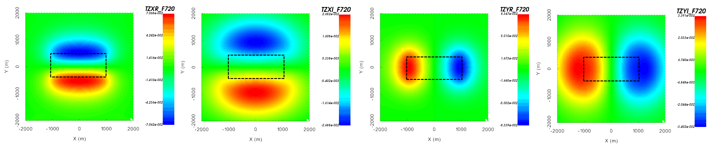
At lower frequencies, ZTEM anomalies are broader. At higher frequencies, ZTEM anomalies are more compact.

\(T_{zx}\) is sensitive to the North and South faces of the conductor while \(T_{zy}\) is sensitive to the East and West faces.

The real component of \(T_{zx}\) is always +ve to the North of the block and -ve to the South of the block.

The real component of \(T_{zy}\) is always +ve to the East of the block and -ve to the West of the block.

For a \(-i\omega t\) Fourier convention (UBC-GIF), the real and imaginary components of the \(T_{zx}\) anomaly will generally have opposing sign at low frequencies (see below at 30 Hz); likewise for the real and imaginary components of \(T_{zy}\). However because of the complicated nature of ZTEM anomalies, this is not true 100% of the time. If possible, determine the Fourier convention from the contractor.

At sufficiently high frequencies, the imaginary component of the anomaly may undergo a change in polarity (see below). This occurs when EM induction effects become larger than the galvanic effects that dominate at lower frequencies.

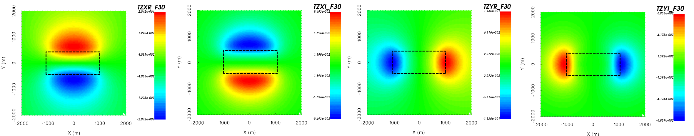
../../../_images/conductor_anomaly_30Hz.png — ZTEM anomaly over a compact conductor at 30 Hz. From left to right: Re[Tzx], Im[Tzx], Re[Tzy] and Im[Tzy].

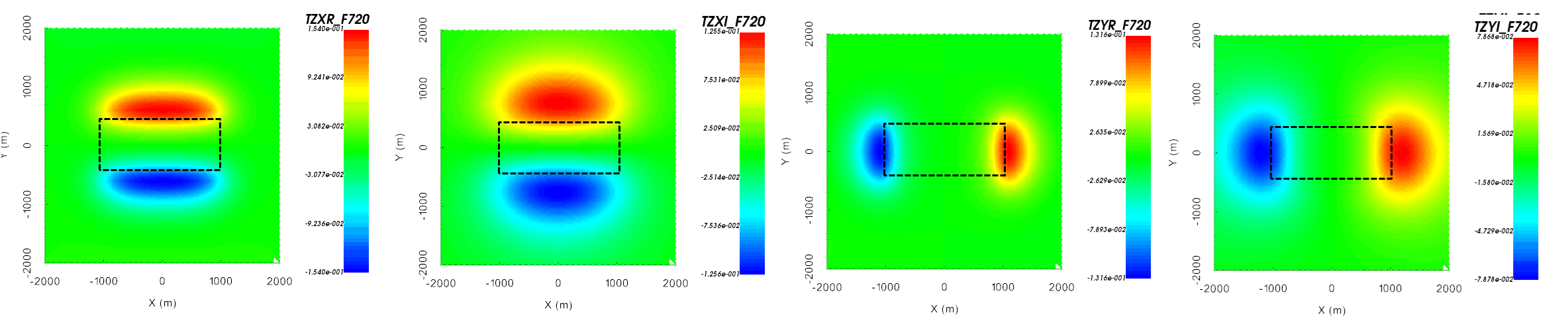
../../../_images/conductor_anomaly_720Hz.png — ZTEM anomaly over a compact conductor at 720 Hz. From left to right: Re[Tzx], Im[Tzx], Re[Tzy] and Im[Tzy].

10.4.1.4. Anomaly over a compact resistor

Let us work again in the UBC-GIF ZTEM data convention; where X is Northing, Y is Easting and Z is +ve downward. The real and imaginary components of the \(T_{zx}\) and \(T_{zy}\) anomalies over a resistive block are shown below. The resistor is buried at a depth of 200 m. Its East-West dimension is 2000 m and its North-South dimension is 1000 m. The background conductivity is 0.001 S/m and the conductivity of the block is 0.1 S/m. We can see that:

The response near the edges of the resistor is large and the response directly over the resistor is relatively small; as ZTEM measurements are sensitive to lateral changes in conductivity and not the conductor itself.

\(T_{zx}\) is sensitive to the North and South faces of the conductor while \(T_{zy}\) is sensitive to the East and West faces.

The real component of \(T_{zx}\) is always +ve to the North of the block and -ve to the South of the block.

The real component of \(T_{zy}\) is always +ve to the East of the block and -ve to the West of the block.

For a \(-i\omega t\) Fourier convention (UBC-GIF), the real and imaginary components of the \(T_{zx}\) anomaly will generally have opposing sign at low frequencies (see below at 30 Hz); likewise for the real and imaginary components of \(T_{zy}\). However because of the complicated nature of ZTEM anomalies, this is not true 100% of the time. If possible, determine the Fourier convention from the contractor.

At sufficiently high frequencies, the imaginary component of the anomaly may undergo a change in polarity (see below). This occurs when EM induction effects become larger than the galvanic effects that dominate at lower frequencies.

../../../_images/resistor_anomaly_30Hz.png — ZTEM anomaly over a compact resistor at 30 Hz. From left to right: Re[Tzx], Im[Tzx], Re[Tzy] and Im[Tzy].

../../../_images/resistor_anomaly_720Hz.png — ZTEM anomaly over a compact resistor at 720 Hz. From left to right: Re[Tzx], Im[Tzx], Re[Tzy] and Im[Tzy].

10.4.1.5. Spatial Transformation to UBC-GIF convention

Let \(\theta\) be the flight direction (counter-clockwise degrees from Northing). Let \(T_{zx}\) and \(T_{zy}\) be the Tipper data in the UBC-GIF coordinate system. And let \(T_{x'}\) and \(T_{y'}\) be the Tipper data in the field data coordinate system. To go from standard airborne data convention to UBC-GIF, the following transformation can be done:

\[\begin{split}\begin{bmatrix} T_{zx} \\ T_{zy} \end{bmatrix} = - \begin{bmatrix} 1 & 0 \\ 0 & -1 \end{bmatrix} \begin{bmatrix} cos \theta & -sin\theta \\ sin\theta & cos\theta \end{bmatrix} \begin{bmatrix} T_{zx'} \\ T_{zy'} \end{bmatrix}\end{split}\]

The operations being performed can be summarized as follows:

The rotation matrix is applied to rotate from flight orientation to Northing (if necessary).

The diagonal matrix transforms the cross-line direction from being 90 degrees counter clockwise relative to along-line direction, to being 90 degrees clockwise relative to along-line direction (if necessary).

The negative sign out front transform the coordinate system from being z +ve upwards to z +ve downwards (if necessary).

Note

This transformation has been built into GIFtools. We will demonstrate this in the workflow.

Note

If the Fourier convention of the the field collected data is not the same as UBC-GIF convention, the imaginary components of the Tipper data can be multiplied by -1 after the coordinate system transform is carried out.

10.4.1.5.1. Example

When ZTEM data are acquired, the contractor will frequently provide the cross-over polarity for data collected along each flight direction (see below). Essentially, they provide the expected Re[Tzx] anomaly, at sufficiently low frequency, over a compact conductor. Given this information, how do we determine the transformation required to go from the field coordinate system to UBC-GIF?

In the figure below, we see the cross-over polarity for a survey that has data collected along two different flight line directions. We will deduce the transformation required to go from the field data coordinate system to UBC-GIF.

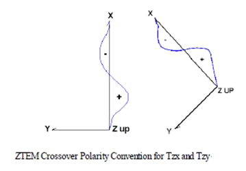
../../../_images/crossover_polarization.png — Convention for airborne data collected along 2 flight bearings.

Z +ve upward or Z +ve downward?

From the figure, we see that the coordinate system for field collected data is defined using a z +ve upward convention, whereas UBC GIF uses a z +ve downward convention. Thus we will need to include this in our transformation.

Is cross-line 90 degrees clockwise or 90 degrees counter clockwise from the along-line direction?

From the figure, we see that the cross-line direction is 90 degrees counter clockwise from the along-line direction. UBC-GIF is 90 clockwise. Thus we will need to include this in our transformation.

What is the flight line direction (along-line direction)?

According to the contractor, I would see +ve Re[Tzx] values followed by -ve Re[Tzx] values if I flew from South to North. Given that data are currently defined with z +ve upward, I know the bearing for this data is 0 degrees. I do not need to rotate the data collected South-North.

Flying Southeast to Northwest, I would see +ve Re[Tzx] values followed by -ve Re[Tzx] values as I fly over the conductor. Given that data are currently defined with z +ve upward, I know the bearing for this data is -45 degrees. I must therefore rotate these data by +45 degrees.

10.4.1.6. Interpretation using total divergence

Tipper data are sensitive to lateral changes in electrical conductivity. To represent the tipper data in a way that is directly sensitive to conductive and resistive structures, we can compute the total divergence parameter (termed the ‘DT’). For both the real and imaginary components, the total divergence parameter is computed by:

\[DT = \frac{\partial T_{zx}}{\partial x} + \frac{\partial T_{zy}}{\partial y}\]

where X = Northing and Y = Easting in the UBC-GIF convention. Below, we plot the total divergence parameter for the real component at 30 Hz over a conductive block and over a resistive block. In these plots, we see that:

A positive anomaly is present for the real component over the conductive block

A negative anomaly is present for the real component over the resistive block

The dimensions of the anomaly are similar to those of the conductor/resistor for simple geometries

../../../_images/total_divergence_30Hz.png — Total divergence of the real component over a conductor at 30 Hz (left). Total divergence of the real component over a resistor at 30 Hz (right).