6.2. The Objective Function
Geophysical inversion recovers a physical property model which fits the data and has geologically reasonable structures. But how is this done in practice? The majority of geophysical inversion algorithms work by minimizing an objective function (\(\phi\)) with respect to the physical property model (\(\mathbf{m}\)):
This is sometimes referred to as “penalty-based optimization”; that is, the objective function is large if the model doesn’t fit the data and/or has implausible structures. The objective function is comprised of three components:
data misfit \(\phi_d (\mathbf{m})\), which is responsible for ensuring the recovered model predicts data that fits the set of field observations.
model objective function \(\phi_m (\mathbf{m})\), which ensures that the recovered model contains plausible geological structures.
trade-off parameter \(\beta\), which weights the relative contribution of \(\phi_d (\mathbf{m})\) and \(\phi_m (\mathbf{m})\) towards the objective function.
Data Misfit:
The Data misfit (\(\phi_d\)) in (1) is given by:
where
\(\mathbf{F[m]}\) is the forward modeling operator; i.e. an operation that predicts the data for a given physical property model \(\mathbf{m}\).
\(\mathbf{d}\) is the set of observed data.
\(\mathbf{W_d}\) is a matrix which weights the difference in predicted and observed data by the data uncertainty. The uncertainty acts as an estimate of the standard deviation of random noise on each data point.
The \(\mathbf{W_d}\) matrix is used for two reasons. 1) If the observed data span several orders of magnitude, we want to make sure that the inversion doesn’t focus on fitting the large values at the expense of the small values. 2) If the noise on our data are independent and Gaussian, then the predicted data fits the noise to an appropriate tolerance when \(\phi_d\) equals the number of data; that is, the inversion fits the signal without fitting the noise (over-fitting). As a result, we generally stop the algorithm when the data misfit is equal to the number of data (target misfit).
Model Objective Function/Regularization:
The model objective function (\(\phi_m\)) is where we impose structures on the recovered model. It also acts as a regularizer; i.e. stabilizes the inversion algorithm. The model objective function can be divided in two sections, the smallness and the smoothness:
With:
\(\phi_{small}\) is the Smallness term. It defines how the model can vary from the reference model \(\mathbf{m}_{ref}\) ((4)).
And:
\(\phi_{smooth}\) is the Smoothness term. it defines how the gradients in each direction, defined by the matrices \(G_x\), \(G_y\) and \(G_z\), of the model can vary from the gradient of the reference model ((5)).
The weighting matrices \(\mathbf{W}_s\), \(\mathbf{W}_x\), \(\mathbf{W}_y\) and \(\mathbf{W}_z\) are cell-specific weightings for each of these terms. They can combine user-defined confidence models with depth or distance weighting.
the alphas parameters \(\alpha_s\), \(\alpha_x\), \(\alpha_y\), and \(\alpha_z\) control how important each of the four terms are relative to each other
The sparsity weights \(\mathbf{R}_s\), \(\mathbf{R}_x\), \(\mathbf{R}_y\) and \(\mathbf{R}_z\) are defined by the lp-norms.
In the UBC codes, the option SMOOTH_MOD_DIFF uses the reference model in all terms, while SMOOTH_MOD would only use the reference model in the Smallness term.
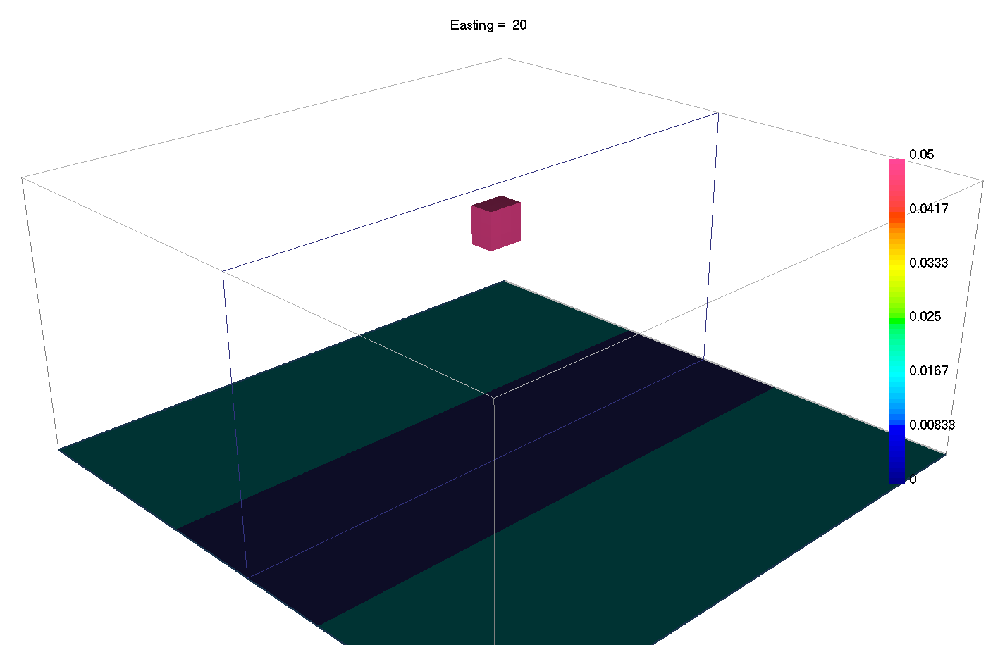
In this section, we will explore the effect of these different parameters on the recovered model through a susceptible block in a non-susceptible half-space mapped with a total magnetic ground survey.