10.3.6. MT Inversion
Here, we provide the steps for setting up and running an inversion with E3DMT or E3DMT v2. We then discuss some important aspects of choosing inversion parameters.
10.3.6.1. Reducing Artifacts through Interface Weighting
When inverting MT data, the E3DMT codes have a tendency to place conductive structures near receiver locations due to the sensitivity of the data to those cells. Here, we generate interface weights to counteract this problem. By forcing lateral smoothness within the top few layers of cells, we can limit the artifacts and force the inversion to place conductive structures at the appropriate depths.
Use edit options and set the following parameters:
set the OcTree mesh
set as log model
set topography as the active cells model
set number of layers and corresponding weights (choose something exponentially decreasing. We chose 100, 20, and 4)
Face value = 0.01
Face tolerance = 0.01
10.3.6.2. Create and Run Inversion
We can now invert MT data using E3DMT v1 or v2.
For the dataset provided, we chose to invert using E3DMT v2, as we were able to define the receiver loops. Things are effectively the same for E3DMT v1. The parameters used are shown below. Note that we must choose the data object that has shifted locations relative to discretized topography.
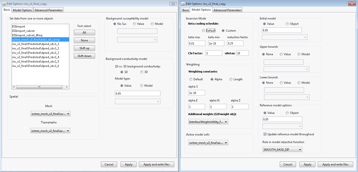
Parameters used to invert the field dataset using E3DMT v2.
10.3.6.3. Discussion of Parameters
Note
The parameters chosen for inversion of the tutorial data set were experimentally derived. The numbers used here worked well for inverting this dataset but should not necessary be used as general default values!
Regarding beta cooling schedule:
For synthetic modeling, we know the uncertainties on our data. With real data, we cannot be 100% sure that we have correctly estimated the uncertainties. In the case that we have globally under-estimated our uncertainties, we sometime set the chi factor to be less than 1. That way, we get to see more of the Tikhonov curve.
When setting the cooling schedule for the tutorial data set, the strategy was pretty straight-forward:
beta max = 0.01. The model recovered at the first iteration should clearly underfit the data. However if beta max is too large, you will have multiple iterations where the model doesn’t budge because no emphasis is being put on fitting the data. We knew a good starting beta for the final inversion from cursory inversions of the data.
beta min = 1e-10. This can be set quite low. But it is good for the inversion to terminate within a reasonable number of beta iterations if target misfit is not reached.
reduction factor = 0.25: We choose a value between 0.1 and 0.9. If the reduction factor is too large, the code will run for a long time since the reduction in beta at each iteration is small. If the reduction factor is too small, we do not get much detail regarding the convergence of the inversion.
chi factor = 1 Here, we assume that appropriate uncertainties are set on the data. Thus, we assume the recovered model explains the data without over-fitting (fitting the noise) when the data misfit equals the number of data observations (chi factor = 1). In practice, you may choose a chi factor less than 1. This will allow you to get a better understanding of the convergence, especially if you have over-estimated the uncertainties.
Regarding the alpha parameters:
As a default setting, we frequently let \(\alpha_x = \alpha_y = \alpha_z = 1\) and we let \(alpha_s = 1/dh^2\) ; where \(dh\) is the width of the smallest cells in the mesh. This effectively balances the emphasis on recovering a model that is similar to a reference model, and recovering a model that has sufficient structure. If we have high confidence in our reference model, we may choose to increase \(\alpha_s\) relative to \(\alpha_x\), \(\alpha_y\) and \(\alpha_z\). If we have low confidence in our reference model, we may choose to decrease \(\alpha_s\) relative to \(\alpha_x\), \(\alpha_y\) and \(\alpha_z\)
For this exercise, we have been able to infer the range of resistivities for this region from apparent resistivity maps and sounding curves. However, we could not identify a consistent background resistivity that works throughout the whole region. As a result, we have set \(\alpha_s = 10^{-10}\) and let \(\alpha_x = \alpha_y = \alpha_z = 1\). This will recover a conductivity model which is primarily driven by the data, and is impacted minimally by the reference model.
Regarding the background, starting and reference models
For the background, starting and reference models, we chose 0.05 S/m. This value was inferred from the apparent resistivity maps and sounding curves over the range of frequencies we are inverting.