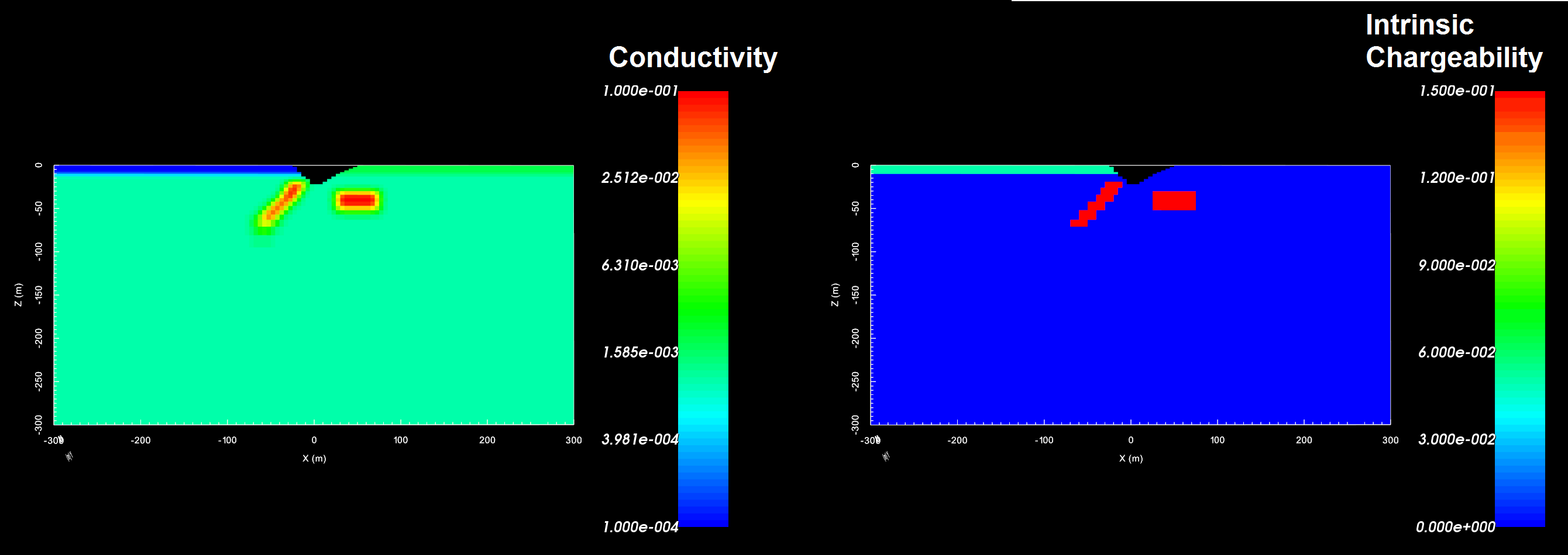
In this recipe, we demonstrate the 2-step processes of inverting 2D DC and IP data. DC data can be inverted without a background model, however IP data a background conductivity. This recipe has 3 steps:
To invert DC data and load the results into GIFtools, carry out the following steps:
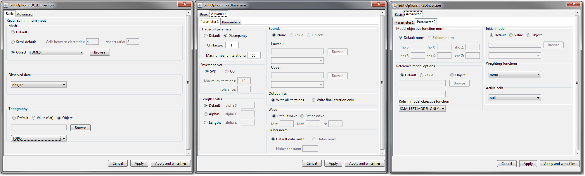
Create 2D DC inversion object: The inversion object is created to provide a single item that 1) contains all parameters relevant to the inversion and 2) keeps track of which mesh, data locations etc… are being used in the inversion.
Edit options tabs showing inputs for test example.
Write files: Once everything is set for the inversion, this command is used to write all the input files for the Fortran code into the specified directory. If you have not set the working (output) directory or would like to change the working directory, use set working directory.
Run the inversion: The forward model can be run directly from GIFtools using the inversion object.
Load results: Once completed, GIFtools can be used to the predicted data and models for each iteration. Since the results are unique to the inversion object, the results are loaded into that folder.
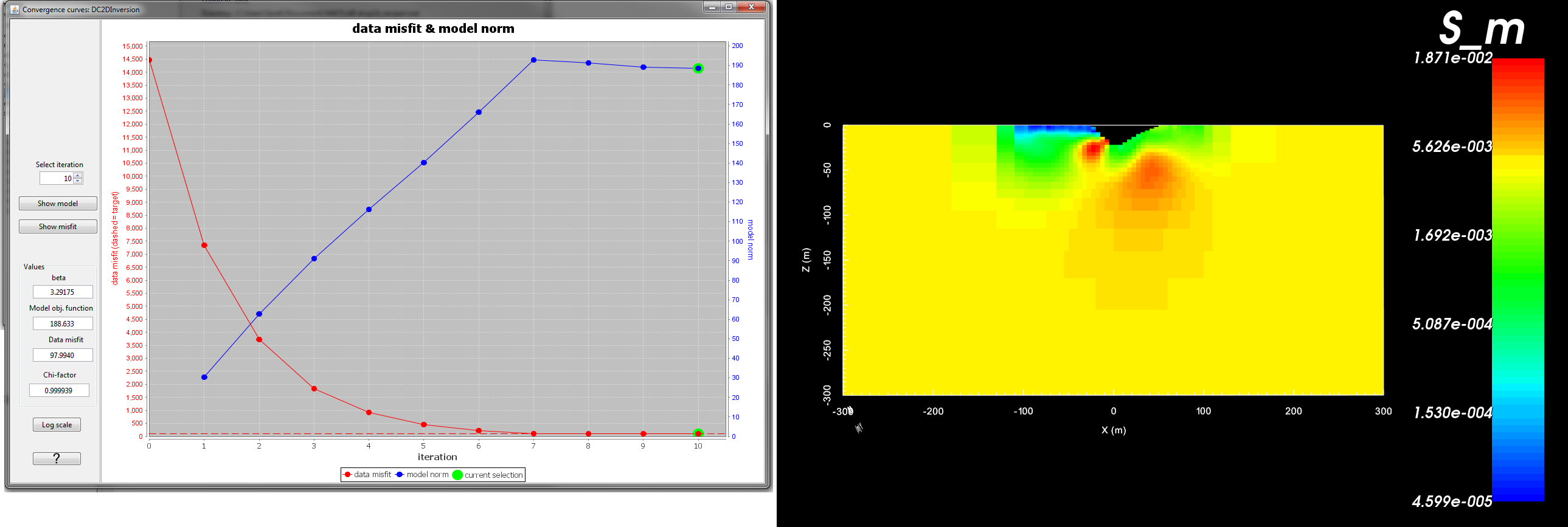
Examine convergence curves, model and misfit maps: Once the inversion has terminated, it is beneficial to examine the convergence towards the final model. This analysis will indicate whether the inversion has hit the target misfit and provide some insight as to whether the assigned data uncertainties were reasonable. The quality of the recovered model can also be assessed by looking at the model itself or the misfit between the predicted and observed data.
Convergence curves (left) and recovered conductivity model - 7th iteration (right) for the test example using the above parameters.
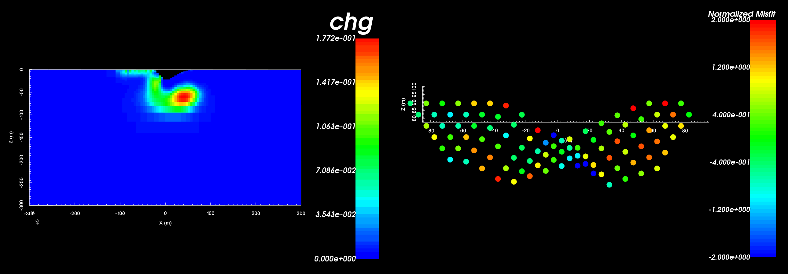
Recovered chargeability model - 8th iteration (left) and corresponding normalize data misfit (right). The chargeability was recovered using the conductivity model from the 7th iteration of the DC invesion.