9.2.3. Magnetic Vector Inversion (MVI)

9.2.3.1. Purpose

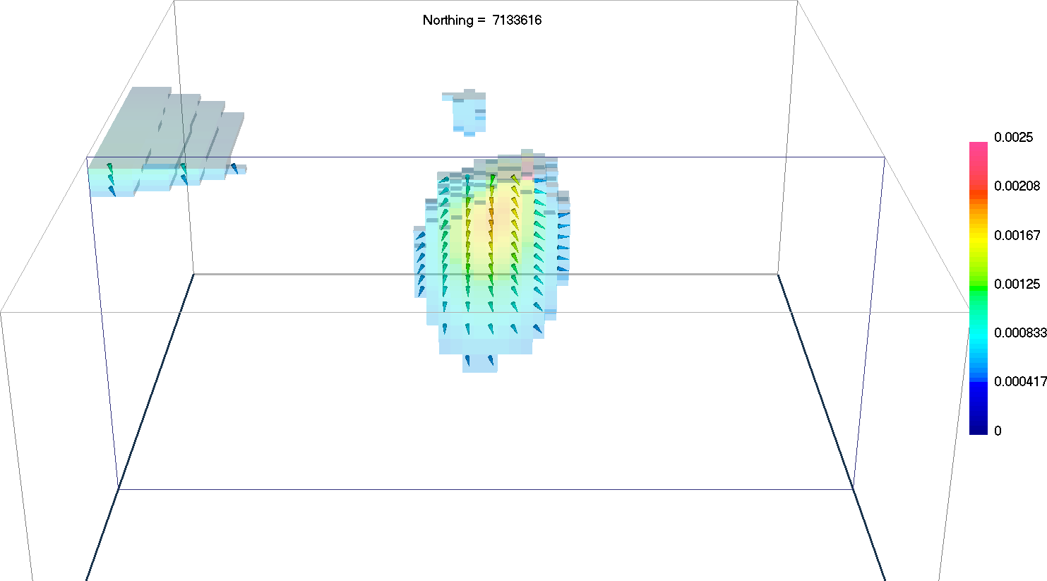
Here, we demonstrate the basic steps for the Magnetic Vector Inversion in both Cartesian (MVI-C) and Spherical (MVI-S) coordinates. We then demonstrate how a cooperative inversion approach (amplitude + MVI-C) can be used to improve the MVI-C solution. Finally we show the advantages of using a sparse MVI-S code.

The true model we will attempt to recover.

Note

Link to MVI documentation

9.2.3.2. Downloads

Example

• Download the demo All files required for this example are located in the sub-folder “MVI”.

• Requires at least GIFtools version 2.25 (July 2018) (login required)

• Requires MVI v3.0 (13062018)

9.2.3.3. Step by step

Tip

If you have already completed either the Magnetic Susceptibility Inversion or the Magnetic Amplitude Inversion demo, you may advance directly to Step 3

• Step 1: Setup

  • Start a GIFtools project

  • Set the working directory

  • Import the topography data from file TKCtopo.dat

  • Import the mesh from file TKC_magSynthetic.msh

• Step 2: Survey and Data

  • Import the processed TMI data in GIF format from the file TKC_magSynthetic_Survey_noIGRF.mag.

Edit options panel 2 for MVI inversion

• Step 3: Processing (NEED IMAGE OF PANELS FILLED OUT)

  • Create an inversion object (MVI v3.0)

  • Edit the options

    • Panel 1: Fill out Sensitivity Options (must use MVI data)

    • Panel 2: Fill out according to the figure on the right

    • Click Apply and write files

• Step 4: Run the inversion: MVI-Cartesian

  • Run all the files

  • Import the inversion results

  • View the convergence curves

Recovered model from MVI inversion

Note

• The magnetic vectors with the highest amplitude are located on the eastern margin of the anomaly.

• Although the direction of magnetization is smoothly changing, the average orientation appears to be pointing downward and towards east.

• We can try to improve this result in two different ways

  1. Re-run cooperatively with the sparse magnetic amplitude model

  2. Run the MVI-Spherical code with sparsity constraints

9.2.3.4. ALTERNATE ENDING #1: Cooperative Magnetic Inversion (CMI)

In this inversion, we will use the compact model obtained in the Magnetic Amplitude Inversion demo to constrain the smooth MVI-C result.

• Copy the inversion object from MVI-C

• Create a cell weighting model \(\mathbf{w}\)

  • Load the final amplitude inversion model file

  • Normalize the amplitude model by its maximum value: \(\mathbf{w} = \mathbf{m}_{amp} / max(\mathbf{m}_{amp})\)

  • Add a small threshold value: \(\mathbf{w} = \mathbf{w}+1e-2\)

  • Apply an inverse power function: \(\mathbf{w} = \mathbf{w}^{-1}\)

  • Assign the cell weights

  

  Cell weights derived from the effective susceptibility model.

• Write all files

• Run the inversion

• Import the last inversion result

Sparse CMI model

9.2.3.5. ALTERNATE ENDING #2: Sparse MVI-Spherical

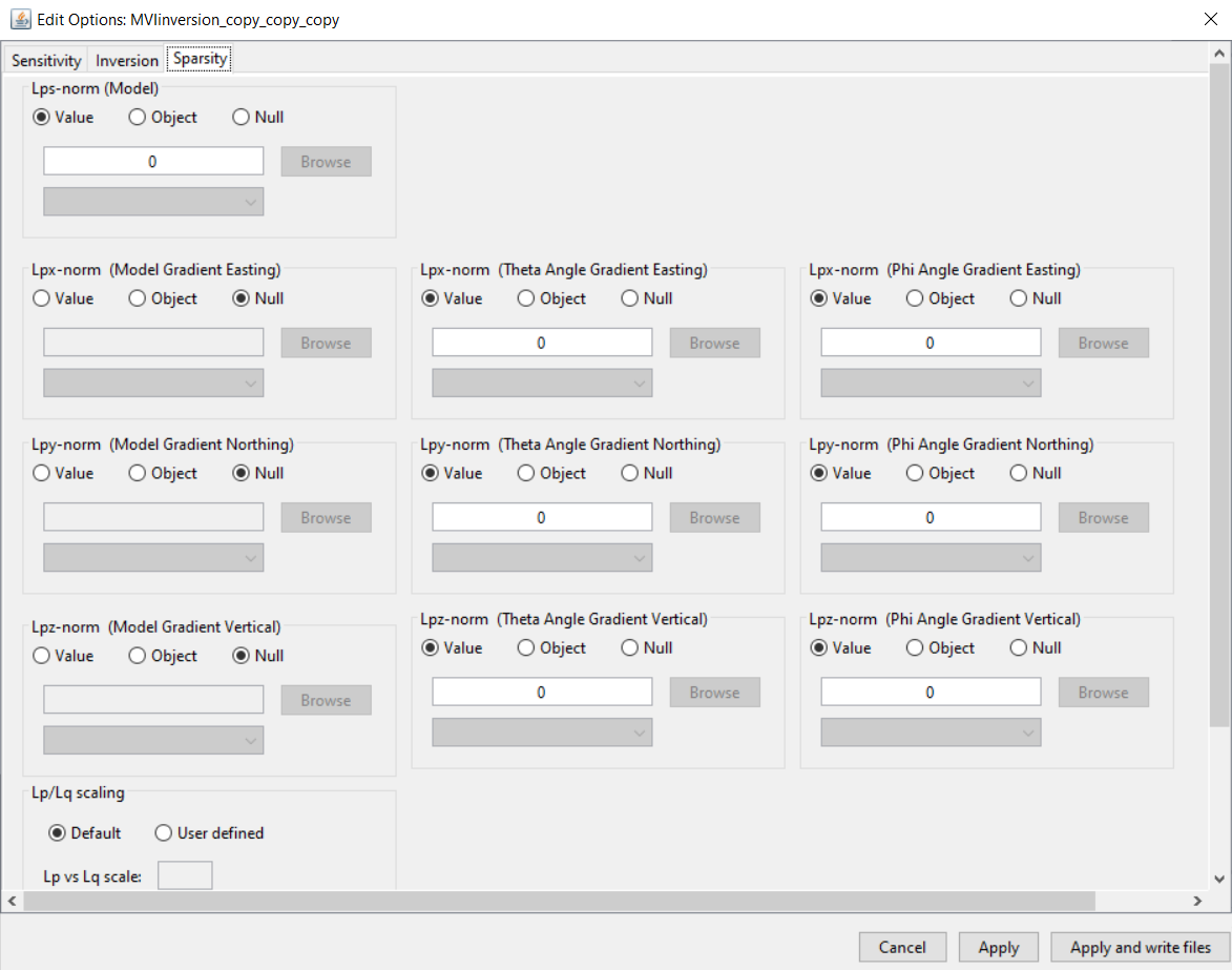
In this inversion, we will use the spherical transformation to apply sparsity on the amplitude and angles independantly. The user is invited to try different combination of norms to test the range of solutions.

• 

• Copy the previous inversion object

• Change the inversion mode to Spherical

• Change the sparsity parameters ->

• Write all files

• Run the inversion

• Import the last inversion result

Sparse MVI-S model

9.2.3.6. Synthesis

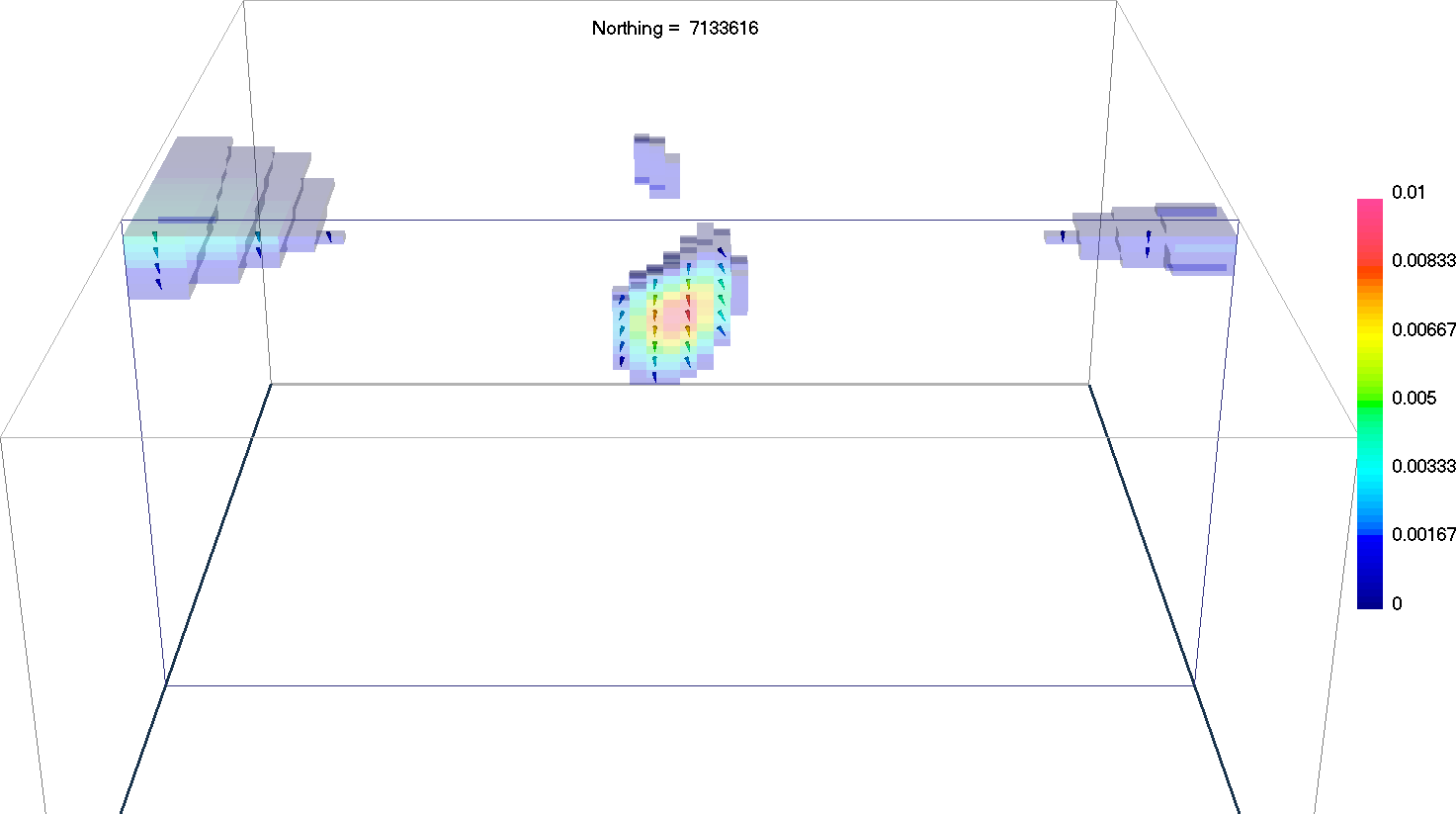
We have recovered three magnetic vector models with the following features:

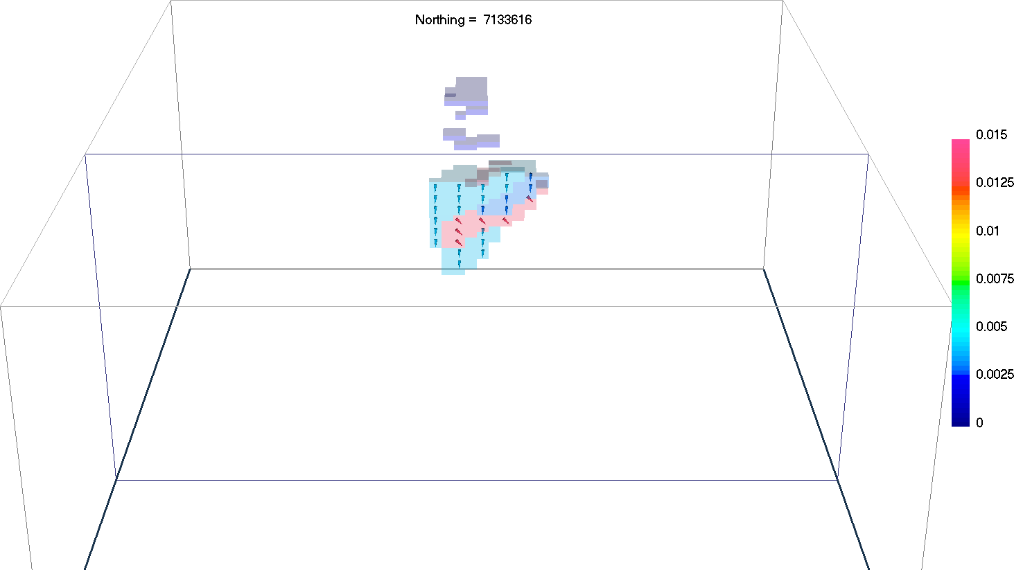
• The MVI-C model was successful in locating the the magnetic kimberlite despite the presence of remanence. Due to the smoothness constraint, the magnetization direction changes throughout the anomaly, making difficult to distinguish a shape or overall trend.

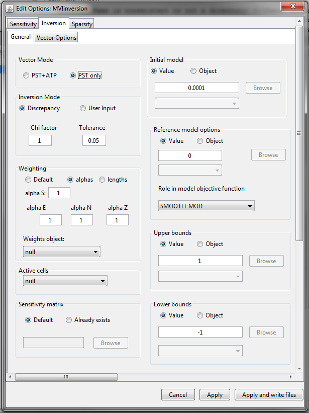
• The Cooperative MVI-C and compact amplitude model dis a better job in imaging a compact body. The magnetization orientation resemble much closely the true model inside the pipe. The horizontal position of the maximum anomaly appears to be slightly shifted West of the true model. This is due assumptions made in the amplitude inversion.

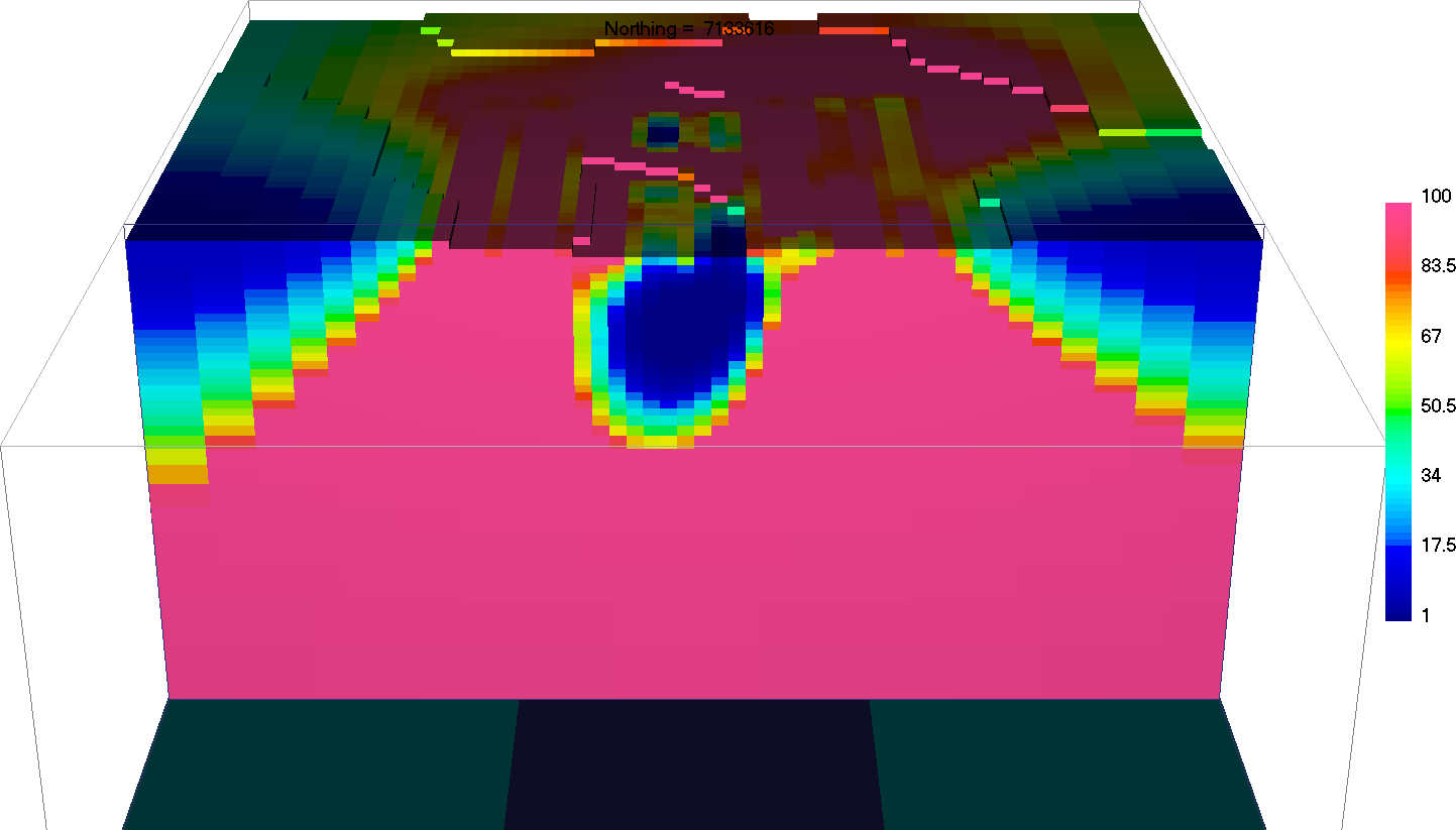
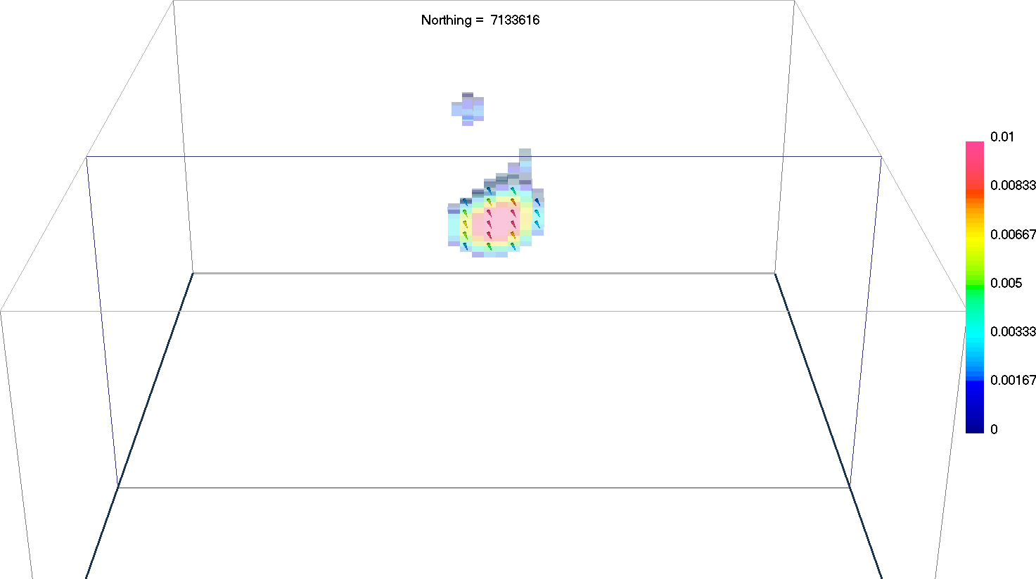
• The sparse MVI-S inversion was arguably the most accurate in recovering both the position and magnetization orientation. Sparsity on the amplitude forced a compact anomaly, while blocky orientation angles allowed for rapid changes in the magnetization direction.

True model Magnetic Vector Inversion: Cartesian (MVI-C) Cooperative Magnetic Inversion (MVI-C + Amplitude) Magnetic Vector Inversion: Spherical (MVI-S)