4.8.2.5. Edit Options for EM1DTM Inversion Objects
This functionality is responsible for setting all inversion parameters pertaining to the EM1DTM code. The list of parameters used to run the EM1DTM Fortran code are described in the EM1DTM package manual; also see inversion methodologies. The edit options window is comprised of 3 tabs:
Global: Sets global inversion parameters such as the 1D mesh, data object, 1D inversion type, model type and computation of the trade-off parameter
Conductivity: specifies the starting model, reference model and regularization for conductivity in the inversion
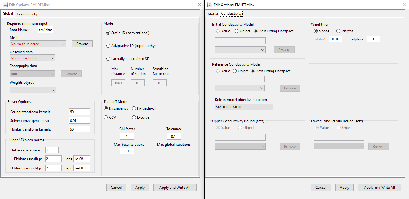
Global (left) and conductivity (middle) tabs for EM1DTM inversion objects.
4.8.2.5.1. Global Tab
Required Minimum Input: Here, the user specifies the:
mesh
observed data
topography (for adaptive and laterally constrained only)
additional model weights (optional)
Model Options: The user may invert for:
a conductivity model
a positive susceptibility model where a static background conductivity is used
conductivity and positive susceptibility models
conductivity and unbounded susceptibility models
Solver Options: Solver options set several parameters used in the EM1DTM Fortran code. The details of each parameters are discussed in the EM1DTM manual
Mode: GIFtools is capable of carrying out three distinct 1D inversion approaches:
Static: Each transmitter is associated with a distinct sounding. The inversion independently recovers a 1D model for each sounding.
Adaptive: Here, surface topography is provided. The inversion is carried out in the same way as before, however the vertical locations of models relative to one another are set based on topography
Laterally constrained: In this approach, the data at each sounding are only sensitive to a particular 1D model. However, the set of 1D models is subject to smoothness constraints in the x and y directions. For this algorithm, three parameters must be set (these parameters are described in the EM1DFM inversion modes):
Max Distance
Number of Stations
Smoothing Factor
For each 1D inversion being run by the EM1DTM Fortran code, there are 4 ways in which the trade-off parameter (\(\beta\)) can be calculated. The performance of each trade-off mode is determine by a set of parameters:
- Discrepancy:
Chi Factor and Tolerance: The algorithm will find the \(\beta\) such that the data misfit \(\phi_d\) is within \(N \times (C.F. \, \pm \, Tol)\) where \(N\) is the number of observations, \(C.F.\) is the chi factor and \(Tol\) is the tolerance. Generally a \(C.F.=1\) and \(Tol=0.1\) are used (static and adaptive only)
Initial Chi Factor and Cooling Factor: This chooses the \(\beta\) for the first iteration according to the aforementioned method. In this case the tolerance is set automatically. For each new global iteration, \(\beta_i = \beta_{i-1}/C\), where \(C>1\) is the cooling factor (laterally constrained only)
Max Beta Iterations: Maximum number of new \(\beta\) the algorithm will compute to find best value
Max Global Iterations: Maximum number of iterations for which the laterally constrained inversion will find a new 3D model
- Fixed trade-off:
Beta: For static and adaptive 1D, the user specifies a constant value and the problem is solved using that \(\beta\). For laterally constrained 1D, this represents the initial \(\beta\) value.
Cooling Factor: For each iteration, \(\beta_i = \beta_{i-1}/C\), where \(C>1\) is the cooling factor
Max Beta Iterations: Maximum number of decreases in \(\beta\) the algorithm will use to hit target misfit
Max Global Iterations: Maximum number of iterations for which the laterally constrained inversion will find a new 3D model
- GCV (static and adaptive only):
Max Beta Decrease: Maximum allowable decrease in \(\beta\) for estimated of \(\beta\) using the GCV method
Max Beta Iterations: Maximum number of new \(\beta\) the algorithm will compute to find the best value
- L-curve (static and adaptive only):
Max Beta Decrease: Maximum allowable decrease in \(\beta\) for estimated of \(\beta\) using the L-curve criterion
Max Beta Iterations: Maximum number of new \(\beta\) the algorithm will compute to find the best value
4.8.2.5.2. Conductivity and Susceptibility Tabs
4.8.2.5.3. Inversion Mode
See the EM1DFM inversion modes for more details.