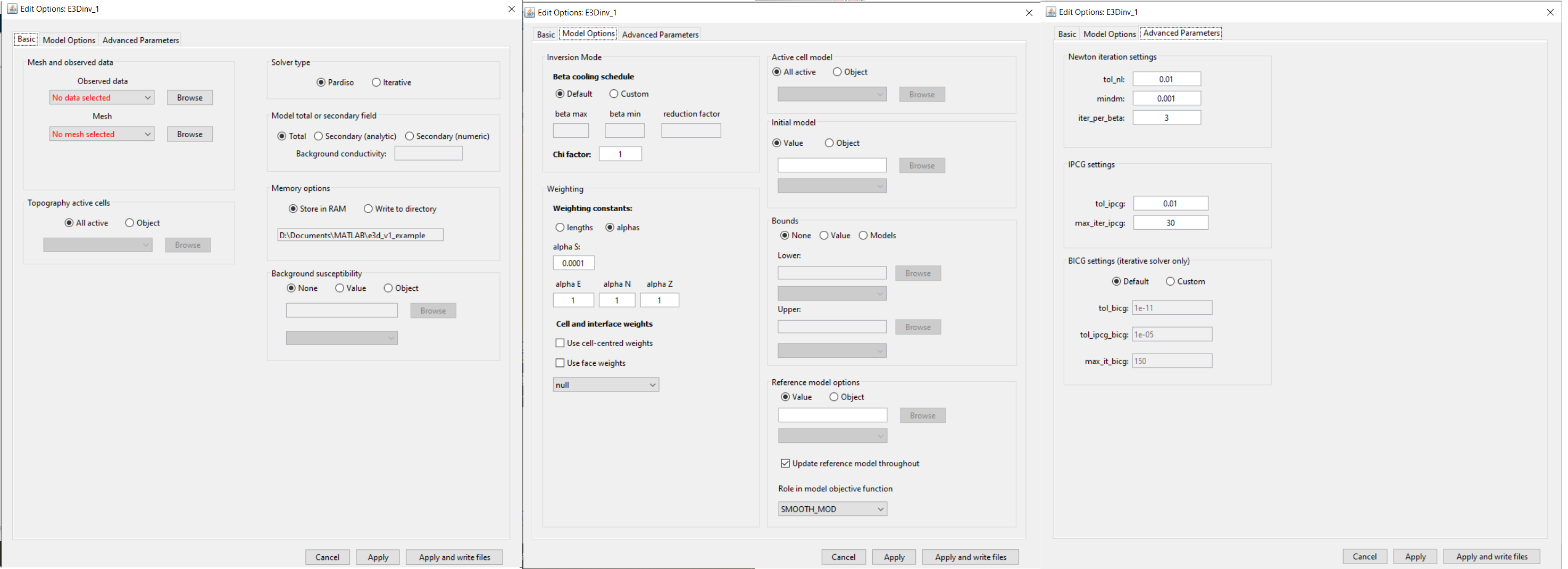
This functionality is responsible for setting all inversion parameters pertaining to the E3D v1 (e3d.exe) and E3DRH v1 code (e3drh.exe); see E3D v1 manual and E3DRH v1 manual . Within the edit options window below, there are 3 tabs:
Basic: Sets minimum required input for the inversion
Model Options: Sets starting model, reference model, upper and lower bounds, weighting constraints and trade-off parameter (beta) options
Inversion Parameters: Sets advanced parameters and tolerances for the inversion
Observed data: The user selects an FEMdata object from the drop-down list.
Mesh: OcTree mesh on which a conductivity model is recovered.
Topography: The user may define the surface topography using an ACTIVEmodel object or set all cells as active (ALL_ACTIVE). If using reference/starting models where air cells are defined as 1e-8 S/m, merely set all topography cells to active. If an ACTIVEmodel is used to define the underground cells, all cells in the air are automatically assigned a value of 1e-8 S/m.
Solver type: The forward problem can be solved with either a direct solver or an iterative solver. The direct solver requires more memory but is faster. The iterative solver is slower but allows the solution of larger problems.
Iterative: Uses the BICGstab algorithm.
Direct: Uses Paradiso
Model total field or secondary field:
Total field: the data output by the forward modeling is the total field.
Secondary (analytic): the code will forward model the secondary field. It will do this by computing the total field for the conductivity model provided, then subtracting the analytic total field using the homogeneous background conductivity provided. To subtract the free-space primary field, let the background conductivity be 1e-8 S/m.
Secondary (numeric): the code will forward model the secondary field. It will do this by computing the total field for the conductivity model provided, then subtracting the numerically computed total field using the homogeneous background conductivity provided. To subtract the free-space primary field, let the background conductivity be 1e-8 S/m.
Background susceptibility model: Here, the user can specify a background magnetic susceptibility model for the inversion. There are 3 options:
No Sus: The Earth is considered non-susceptible
Value: A constant magnetic susceptibility value is assigned to all cells lying below the surface topography (not currently implemented)
Beta Cooling Schedule: Sets the rate of decrease in beta as the algorithm puts increasing emphasis on fitting the data; see fundamentals of inversion.
Default: A default cooling schedule is used.
Custom: The user sets the following parameters:
beta max: Starting beta value
beta min: Final beta value before the algorithm quits (if target misfit not attained)
reduction factor: a multiplicative constant between (0,1). Sets how much beta is reduced at each iteration
Chi Factor: Sets the target data misfit for the inversion. A chi-factor of 1 (default value) implies the data misfit is equal to the total number of data observations.
Weighting constants: Sets the weights for smallness and smoothness regularization in x, y and z; see fundamentals of inversion.
Default: Sets the values of alpha S, alpha E, alpha N and alpha Z based on cell dimensions
Alphas: Sets specific values for alpha S, alpha E, alpha N and alpha Z
Lengths: User sets values Len E, Len N and Len Z which define the values of alpha X, alpha Y and alpha Z relative to alpha S. These relationships are given by \(L_E = \sqrt{\frac{\alpha_E}{\alpha_S}}\), \(L_N = \sqrt{\frac{\alpha_N}{\alpha_S}}\) and \(L_Z = \sqrt{\frac{\alpha_Z}{\alpha_S}}\).
Additional weights: Here, the user may specify the implementation of additional cell and/or face weighting; see fundamentals of inversion. In this case, the user selects a GIFweight object that is defined on the OcTree mesh.
Active model cells: Here, the user specifies which cells are active during the inversion (allowed to change their value). If all are set to active, then all cells within the surface topography are allowed to change. If an active cells model is used, only the active cells change their value during the inversion; the remaining cells (inactive) are left as the starting model value.
Initial model: Staring model for the inversion. Can be either a constant value or an OcTree model
Upper bounds: Upper bounds for the recovered conductivity model.
None: No upper bounds
Value: Set a constant upper bound to be applied to all cells.
Model: An OcTree model that defines the upper bound for each cell individually. Values corresponding to inactive cells in the inversion are ignored.
Lower bounds:
None: No lower bounds
Value: Set a constant lower bound to be applied to all cells.
Model: An OcTree model that defines the lower bound for each cell individually. Values corresponding to inactive cells in the inversion are ignored.
Value: Set a constant value for the reference model.
Model: An OcTree model that defines the reference model.
Update reference model throughout:
Un-checked: The reference model remains the same throughout the entire inversion. This option emphasizes preserving structures included in the reference model.
Checked: Each time beta is updated, the current recovered model is set as the reference model for the next beta value. This results in faster convergence but does not emphasize preserving structures in the original reference model as strongly.
Newton iteration settings: Sets stopping criteria for Gauss-Newton iterations; see E3D version 1 manual . Parameters are:
tol_nl: stopping criteria based on gradient size (defaul = 0.01)
mindm: stopping criteria based on size of model perturbation (default = 0.001)
iter_per_beta: maximum number of Gauss-Newton iterations (default = 3)
IPCG settings: Sets tolerances for solving the system at each Gauss-Newton iteration using incomplete preconditioned conjugate gradient; see E3D version 1 manual . Parameters are:
tol_ipcg: relative tolerance for solution (default = 0.01)
max_iter_ipcg: maximum number of IPCG iterations (20)
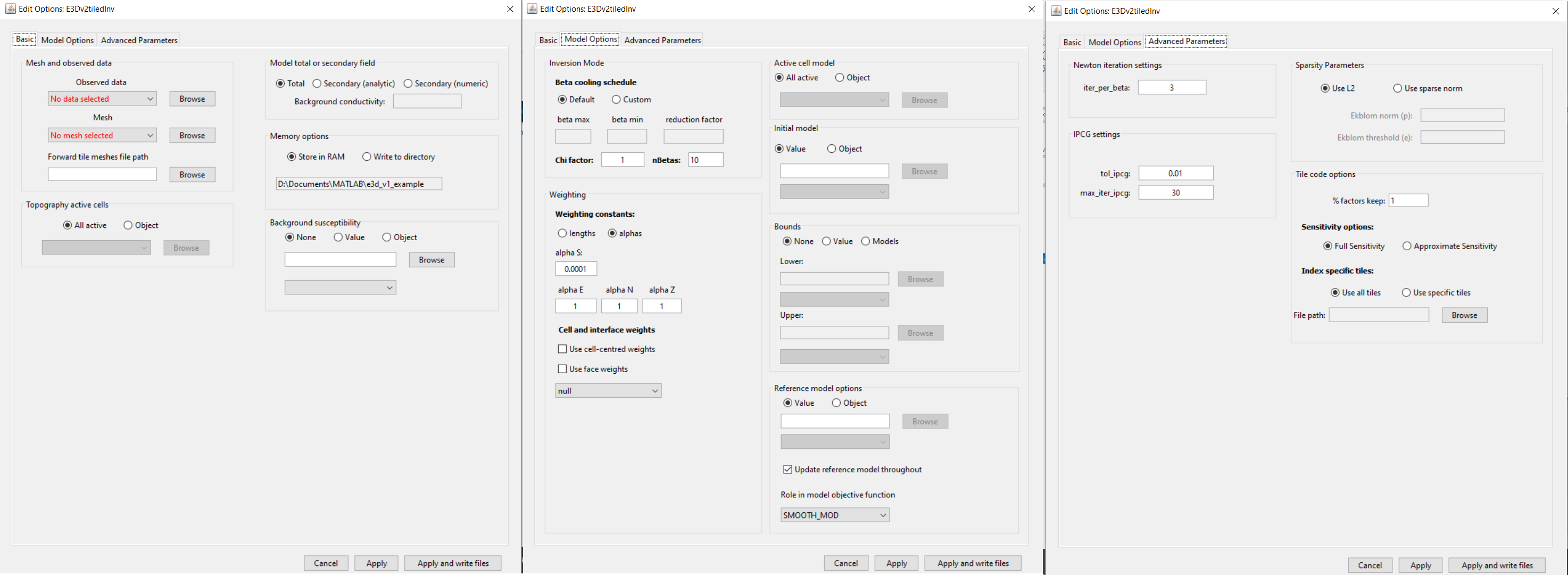
This functionality is responsible for setting all inversion parameters pertaining to the codes: E3D v2 (e3d_v2.exe), E3D v2 tiled (e3d_v2_tiled.exe),
E3DRH v2 (e3drh_v2.exe) and E3DRH v2 tiled (e3drh_v2_tiled.exe). See manuals for E3D v2 , E3D v2 tiled manual , E3DRH v2 and E3DRH v2 tiled manual . Within the edit options window below, the user sets the following parameters for the forward modeling:
Basic: Sets minimum required input for the inversion
Model Options: Sets starting model, reference model, upper and lower bounds, weighting constraints and trade-off parameter (beta) options
Inversion Parameters: Sets advanced parameters and tolerances for the inversion
Observed data: The user selects either and impedance data or ZTEM data object from the drop-box provided.
Mesh: OcTree mesh on which a conductivity model is recovered.
Forward tile meshes file path (tiled code only): Sets the path to the file containing the local meshes (tiles)
Topography: The user may define the surface topography using an ACTIVEmodel object or set all cells as active (ALL_ACTIVE). If using reference/starting models where air cells are defined as 1e-8 S/m, merely set all topography cells to active. If an ACTIVEmodel is used to define the underground cells, all cells in the air are automatically assigned a value of 1e-8 S/m.
Model total field or secondary field:
Total field: the data output by the forward modeling is the total field.
Secondary (analytic): the code will forward model the secondary field. It will do this by computing the total field for the conductivity model provided, then subtracting the analytic total field using the homogeneous background conductivity provided. To subtract the free-space primary field, let the background conductivity be 1e-8 S/m.
Secondary (numeric): the code will forward model the secondary field. It will do this by computing the total field for the conductivity model provided, then subtracting the numerically computed total field using the homogeneous background conductivity provided. To subtract the free-space primary field, let the background conductivity be 1e-8 S/m.
Background susceptibility model: Here, the user can specify a background magnetic susceptibility model for the inversion. There are 3 options:
No Sus: The Earth is considered non-susceptible
Value: A constant magnetic susceptibility value is assigned to all cells lying below the surface topography (not currently implemented)
Beta Cooling Schedule: Sets the rate of decrease in beta as the algorithm puts increasing emphasis on fitting the data; see fundamentals of inversion or E3D v2 manual .
Default: A default cooling schedule is used.
Custom: The user sets the following parameters:
beta max: Starting beta value
beta min: Final beta value before the algorithm quits (if target misfit not attained)
reduction factor: a multiplicative constant between (0,1). Sets how much beta is reduced at each iteration
Chi Factor: Sets the target data misfit for the inversion. A chi-factor of 1 (default value) implies the data misfit is equal to the total number of data observations.
nBetas: Set the maximum number of times that Beta is reduced and the optimization is carried out to recover a new model.
Weighting constants: Sets the weights for smallness and smoothness regularization in x, y and z; see fundamentals of inversion.
Default: Sets the values of alpha S, alpha E, alpha N and alpha Z based on cell dimensions
Alphas: Sets specific values for alpha S, alpha E, alpha N and alpha Z
Lengths: User sets values Len E, Len N and Len Z which define the values of alpha X, alpha Y and alpha Z relative to alpha S. These relationships are given by \(L_E = \sqrt{\frac{\alpha_E}{\alpha_S}}\), \(L_N = \sqrt{\frac{\alpha_N}{\alpha_S}}\) and \(L_Z = \sqrt{\frac{\alpha_Z}{\alpha_S}}\).
Additional weights: Here, the user may specify the implementation of additional cell and/or face weighting; see fundamentals of inversion. In this case, the user selects a GIFweight object that is defined on the OcTree mesh.
Active model cells: Here, the user specifies which cells are active during the inversion (allowed to change their value). If all are set to active, then all cells within the surface topography are allowed to change. If an active cells model is used, only the active cells change their value during the inversion; the remaining cells (inactive) are left as the starting model value.
Initial model: Staring model for the inversion. Can be either a constant value or an OcTree model
Upper bounds: Upper bounds for the recovered conductivity model.
None: No upper bounds
Value: Set a constant upper bound to be applied to all cells.
Model: An OcTree model that defines the upper bound for each cell individually. Values corresponding to inactive cells in the inversion are ignored.
Lower bounds:
None: No lower bounds
Value: Set a constant lower bound to be applied to all cells.
Model: An OcTree model that defines the lower bound for each cell individually. Values corresponding to inactive cells in the inversion are ignored.
Value: Set a constant value for the reference model.
Model: An OcTree model that defines the reference model.
Update reference model throughout:
Un-checked: The reference model remains the same throughout the entire inversion. This option emphasizes preserving structures included in the reference model.
Checked: Each time beta is updated, the current recovered model is set as the reference model for the next beta value. This results in faster convergence but does not emphasize preserving structures in the original reference model as strongly.
Newton iteration settings: Sets stopping criteria for Gauss-Newton iterations; see E3D v2 manual . Parameters are:
tol_nl: stopping criteria based on gradient size (defaul = 0.01)
iter_per_beta: maximum number of Gauss-Newton iterations (default = 3)
IPCG settings: Sets tolerances for solving the system at each Gauss-Newton iteration using incomplete preconditioned conjugate gradient; see E3D v2 manual . Parameters are:
tol_ipcg: relative tolerance for solution (default = 0.01)
max_iter_ipcg: maximum number of IPCG iterations (20)
Memory settings: This code factors the forward system at each frequency for repeated use in the inversion algorithm. The user has a choice in where the factorizations are stored:
Store in RAM: Factorizations are stored in RAM. This option is the fastest, however the user may run into memory limits.
Write to file: Factorizations are written to files. Larger problems can be solved, however the continual reading and writing of files makes this options slower.
Tile code options:
Percent factors keep: A number between 0 and 1 denoting the fractional percent of tiles being used each time the sensitivities are computed.
Sensitivity Options: Compute full sensitivities or approximate
Index specific tiles: Only invert using a subset of the data for the files specified.