9.5.3. 3D Inversion

9.5.3.1. Purpose

In this section, we will invert the simulated data in 3D with three strategies:

• Case 1: Unconstrained inversion

• Case 2: Sensitivity weighted inversion

• Case 3: Inversion with 2D starting model

Note

Link to DCIP3D documentation

9.5.3.2. Downloads

Example

• Download the demo

• Requires at least GIFtools 2.26 (login required)

• Requires DCIP v5

9.5.3.3. Step by step

Tip

If you have already completed either the Survey Design and Simulation or the 2D Inversion demo, you may advance directly to the Unconstrained Inversion Section

• Step 1: Setup

  • Start a GIFtools project

  • Set the working directory

  • Import the topography data

• Step 2: Survey and Data

  • Import the DC data in UBC format

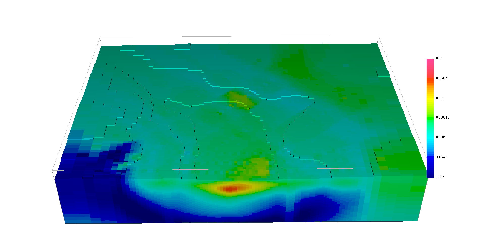
9.5.3.4. Case 1: Unconstrained Inversion

As a first step, we invert the simulated data with a purely unconstrained approach.

• Create an inversion object (DC3Dinversion)

  • Edit the options

    • Panel 2: Adjust \(\alpha\) parameters: \(\alpha_s=0.0025, \alpha_x=\alpha_z=1\)

    • Click Apply and write files

  • Run the inversion

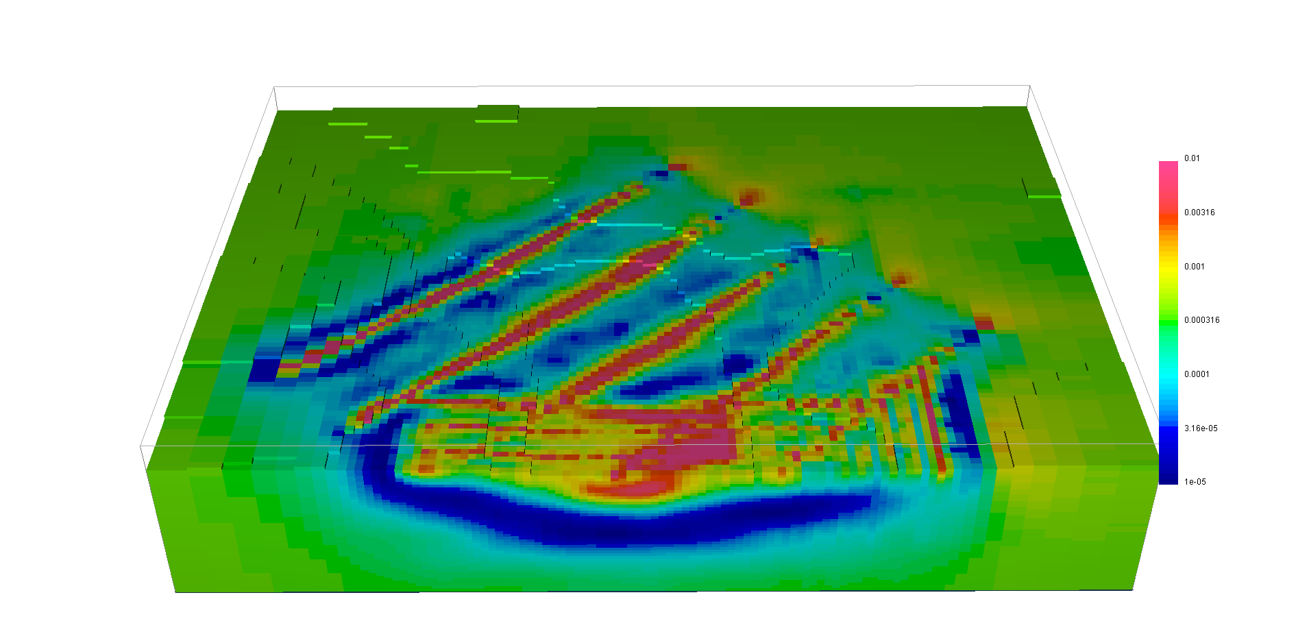
9.5.3.5. Case 2: Sensitivity weighted inversion

The result obtained with the unconstrained approach appears to be dominated by the source-receiver position, with most of the conductivity anomalies recovered near the survey lines. In order to reduce this geometric bias, we will incorporate sensitivity-based weights.

• Copy the inversion object from the previous example

• Load the sensitivity file generated by DCINV3D

• Create sensitivity weight

• Write All and Run

Note

This solution is an improvement over the purely unconstrained as lower conductivity anomalies are recovered at the electrodes, while the conductive kimberlites are better recovered

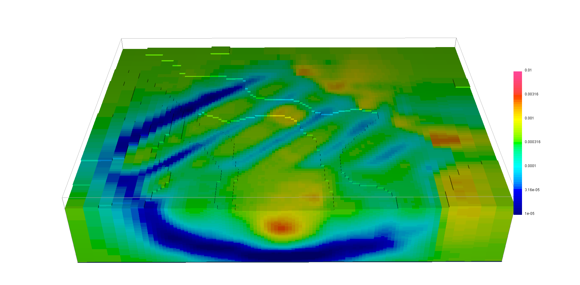
9.5.3.6. Case 3: Inversion with 2D starting model

In the third case, we will incorporate the stiched 2D model in the 3D inversion through a starting and a reference model.

To create a full 3D model from the merge 2D models created in the merging step, the steps are:

• Right-click on the merged model

• Select Edit -> Fill/Interpolate no-data-value (see the documentation)

• Keep the default parameters and enter 1e-8 as no-data-value and choose the Log interpolation

Then you can use that model as starting and reference model:

• Copy the inversion object from Case 2

• Set the reference and starting model

• Write All and Run

Note

We have once again improved the solution, and the iteration process is a lot quicker since we are starting with a model closer to the final solution.