9.3.3. Laterally Constrained 3D Inversion
Here, frequency-domain data are inverted using the laterally constrained 3D inversion approach. Just like in the previous exercise, every 1D model is associated with a distinct sounding location (see EM1DFM package overview). However lateral constraints are added such that the set of recovered 1D models are smooth horizontally and can ultimately be constrained and interpreted in 3D. The laterally constrained 3D inversion algorithm is a computationally fast way to invert FEM data while taking into account both vertical and horizontal variability of the Earth. The final model recovered by this algorithm is fully 3-dimensional.
As part of this exercise, the user will:
9.3.3.1. Setup for the Exercise
If you have completed the tutorial “Static and Adaptive 1D Inversion”:
Open your preexisting GIFtools project
Set the working directory (if you would like to change it)
If you have NOT completed the previous tutorial and would like to start here, complete the following steps:
Open GIFtools
Import em1dfm data file: Assets//FEM1D.obs (1D FEM GIF format data in ppm)
Import 1D mesh (layers file)
Import the topography data (3D GIF format)
- Create elevation from surface topography
Set elevation at 40 m above topography
Set i/o header for Z to the elevation column you just created.
Note
The uncertainties for this exercise are the same as the uncertainties used to invert real FEM data collected over TKC.
 |
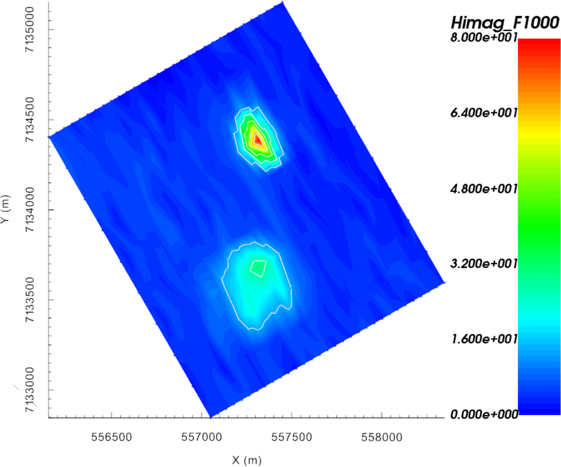 |
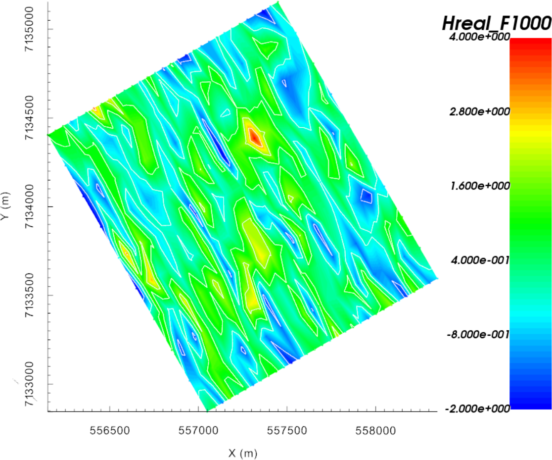
Real (left) and quadrature (right) components of synthetic FEM data collected over TKC
9.3.3.2. Laterally Constrained 3D FEM Inversion
Here, the set of FEM data are inverted using the laterally constrained 3D approach.
9.3.3.2.1. Setup the inversion
If you have completed the tutorial “Static and Adaptive 1D Inversion”:
Click on a preexisting EM1DFM inversion object and copy options
Click on the newly created EM1DFM inversion object to set the output directory
- Set any necessary EM1DFM inversion parameters under edit options:
Make sure the mesh, observed data and topography are properly set!
- Mode: Laterally constrained 3D
Max distance = 1000 m
Number of stations = 10
Smoothing parameter = 200
Other parameters left as default values
- Use the Fix Trade-off mode
Initial beta = 1000
Cooling factor = 5
Global Iterations = 5
Other parameters left as default values
Click Apply
If you have NOT completed the previous tutorial and are starting here:
Create an EM1DFM inversion object and set the output directory
Set the EM1DFM inversion parameters under edit options using the parameters specified in the bullet list above
Click Apply
Note
If you chose not to write the files from the edit options menu, you may do so through write inversion files
9.3.3.2.2. Run Inversion and Load Results
Results are loaded automatically for this algorithm
9.3.3.2.3. Discussion
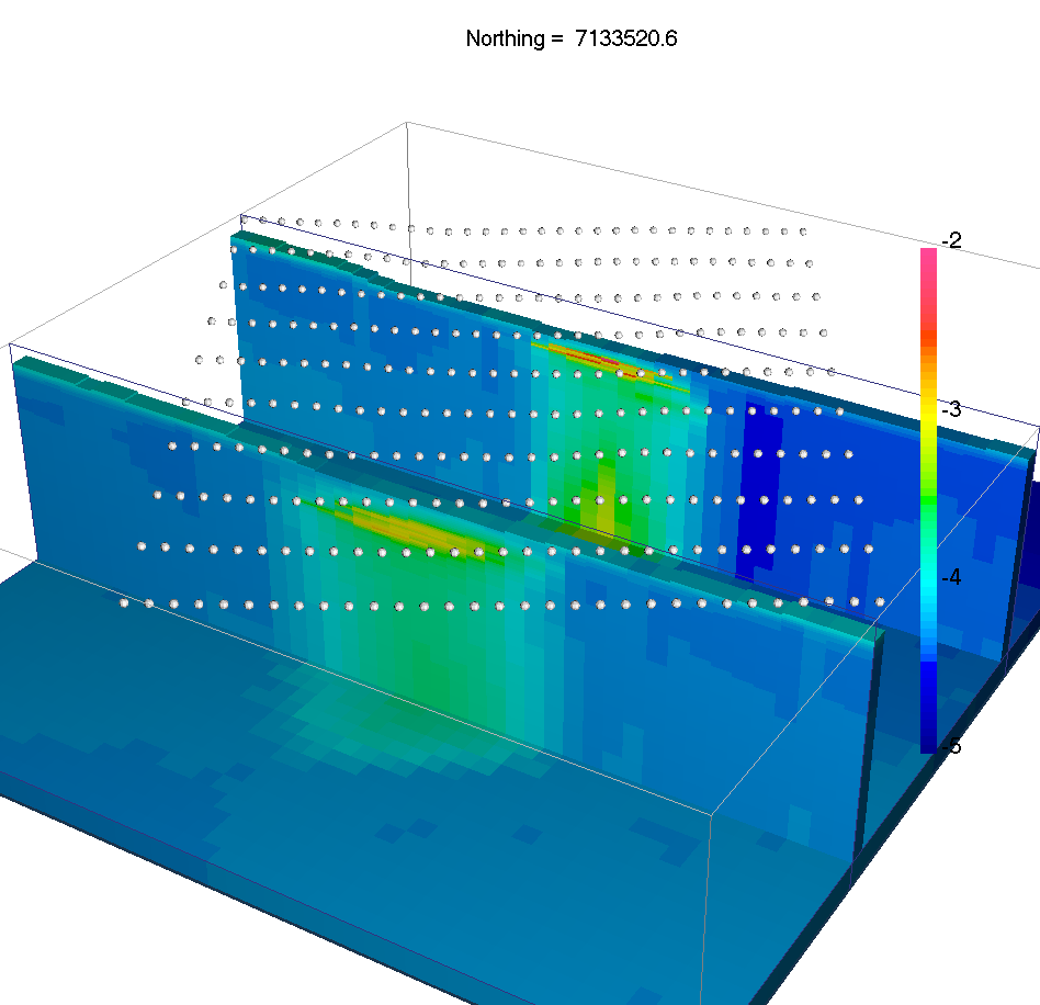
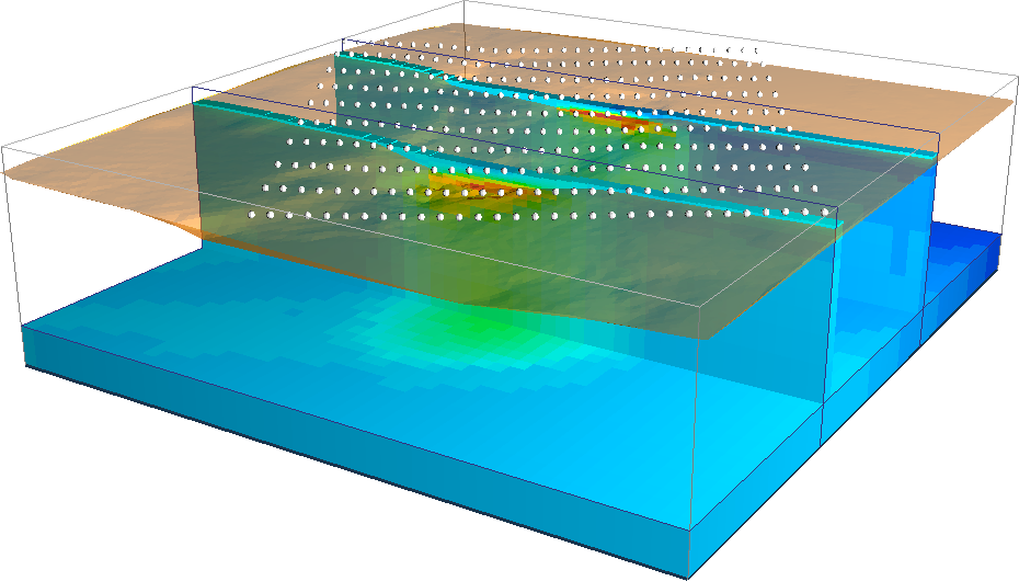
Recovered 1D models with topography and lateral constraints
The lateral constraints strategy comes with many advantages:
Neighboring 1D conductivity models are more consistent
Conductivity structures are interpolated in 3D, possibly highlighting trends in the model and easing the interpretation.
Possible to employ a \(\beta\)-cooling strategy similar to the 3D inversion code.
The use of a global measure of data fit allows us to assess the convergence of the algorithm through the usual convergence curve window.
Ideally we would like to test the hypothesis of a conductive overburden in 3D, as well as to impose bounds on the conductivity values. which we covered in the next section.
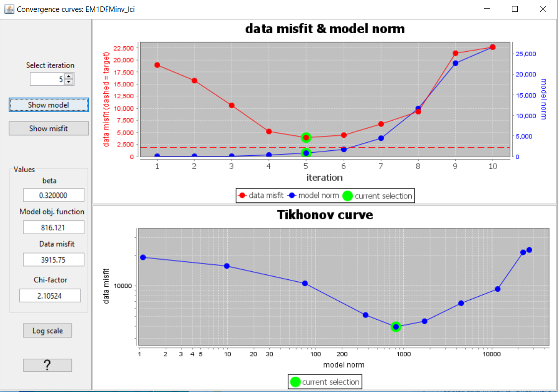
Convergence curves
Note
After the fifth iteration, the global misfit begins to increase due to the 3D smoothing of the recovered conductivity model. The user should consider re-running the inversion with different smoothing parameters in order to test the stability of the solution.
9.3.3.3. Geological Constraints: Hypothesis Testing
It is well known that at TKC, there is a till overburden covering a portion of the survey area. As a final example we will impose 3D geological constraints on the laterally constrained 1D inversions. The geological constraints assume we have some a-priori information about the distribution and thickness of the overlying till. To apply geological constraints, we first need to create the reference conductivity model from a surface:
9.3.3.3.1. Creating a Reference Model
Here, we use surface topography and a surface object to define the upper and lower surfaces of the till layer, respectively. We then assign reasonable physical property values for the till and background. To accomplish this task, we use the model builder module.
Import the surface file provided (TillLayer.topo)
Select one of the 3D mesh objects created from a previous inversion and create active model from topography. Use from tops of cells.
Select the active cells model and create a model builder module
- Create model using surfaces with the following parameters to create an initial physical property model:
Top surface as topography
Bottom surface as surface object
Value as physical property value (set as \(10^{-4}\) S/m)
Destination model as New Model and provide a name (RefMod)
- Setting physical property values for the active background cells in the newly created model can with the same functionality. Open the Create model using surfaces window and use the following parameters
Top surface as surface object
Bottom surface as Value (\(-1000\) m)
Value as physical property value (set as \(10^{-5}\) S/m)
Destination model as the physical property model you just created
This model can be used as a reference model and constrain the final recover conductivity model.
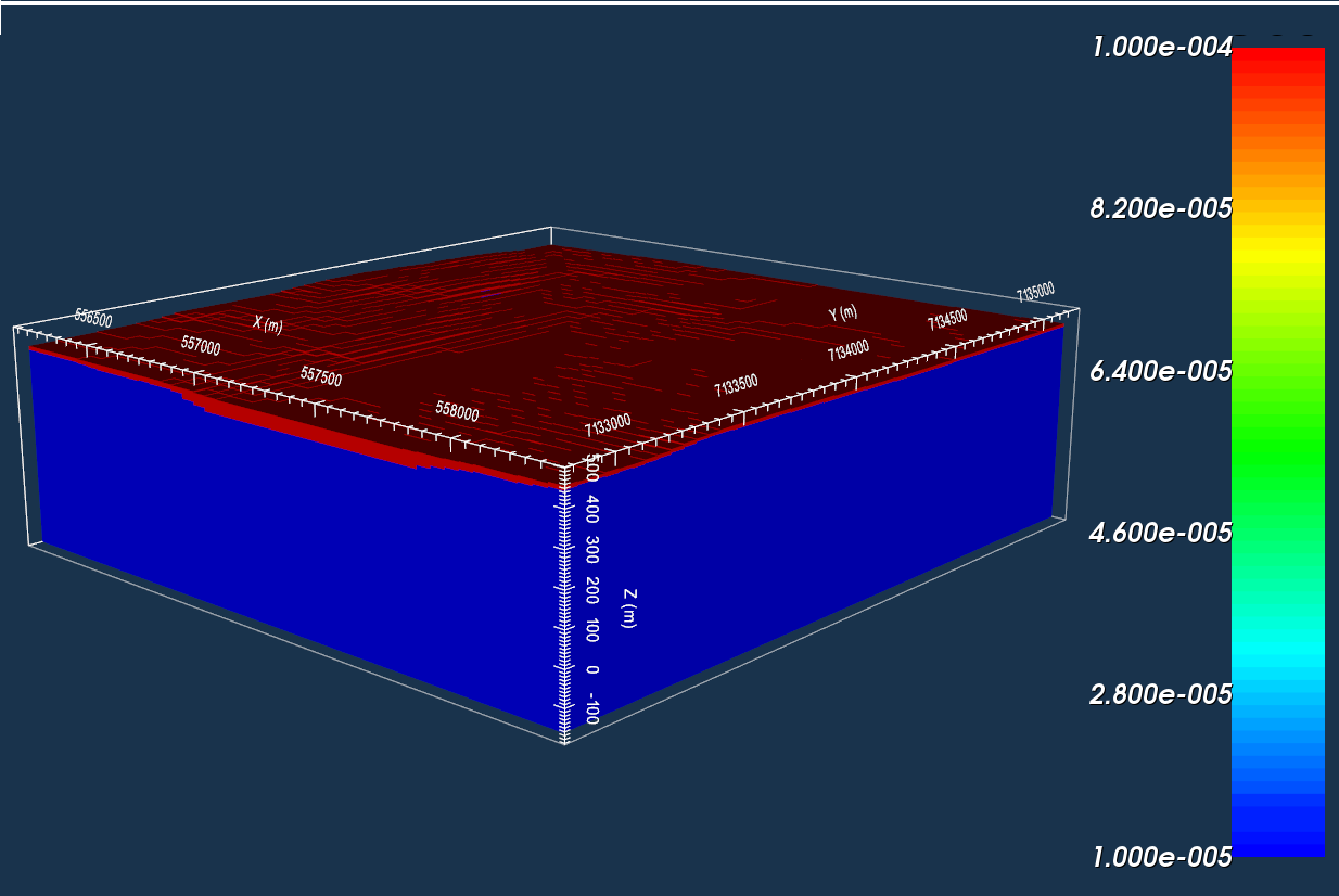
Till layer defined within the reference model.
9.3.3.3.2. Setup the inversion
Click on the last EM1DFM inversion object and copy options
Click on the newly created EM1DFM inversion object and set the output directory
- Use edit options to verify and apply the current set of inversion parameters
Make sure the mesh and observed data are properly set
Set the topography from the drop-down menu
Notice that the inversion parameters are identical to the previous inversion that was run
- Within edit options Conductivity tab, set:
Initial model as best-fitting halfspace
Reference model as the model created in the previous subsection and choose “SMOOTH_MOD_DIF”
Upper and lower bounds for the recovered model can be set if desired
Apply and write all files
9.3.3.3.3. Run Inversion and Load Results
Results are loaded automatically for this algorithm
9.3.3.3.4. Discussion
- This final solution differs from the previous inversion in that:
A sharp gradient is preserved along the base of the till layer
The upper conductivities are more consistent \(\approx 10^4 \Omega \cdot m\)
The top of the kimberlite pipes is at the right depth
The reader is invited to run multiple inversions with various smoothing parameters and data uncertainties to explore the range of solutions. It is important to keep in mind that the true model is 3D and cannot be characterized by the 1D assumption. We did however manage to recover a first order estimate for the horizontal positions of the kimberlite pipes and background conductivity structures.
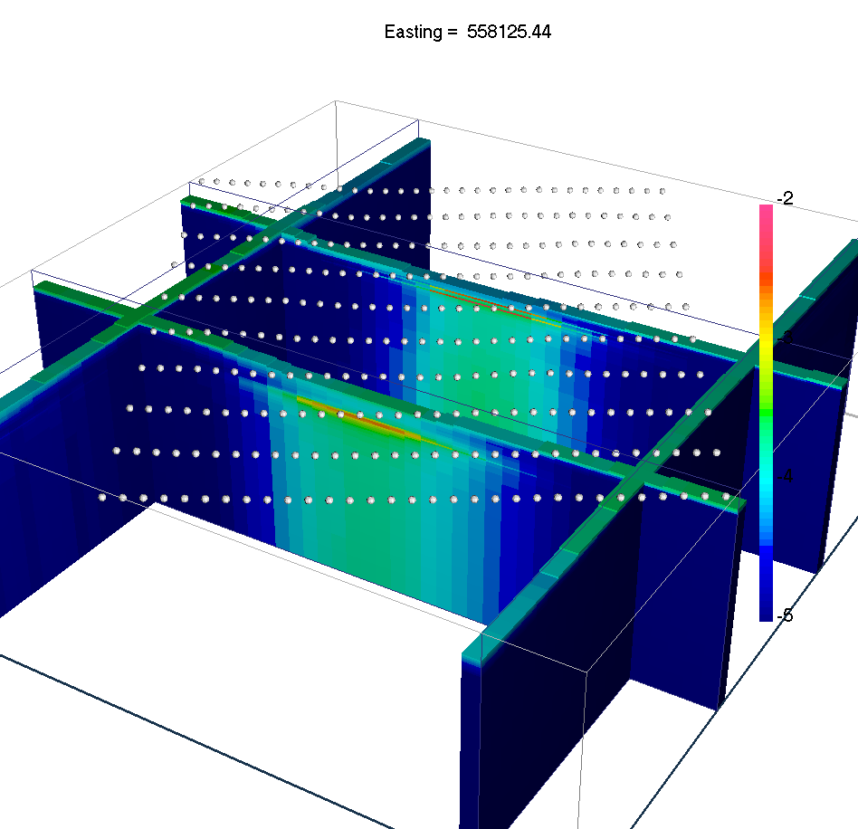
Recovered 1D models with geological constraints
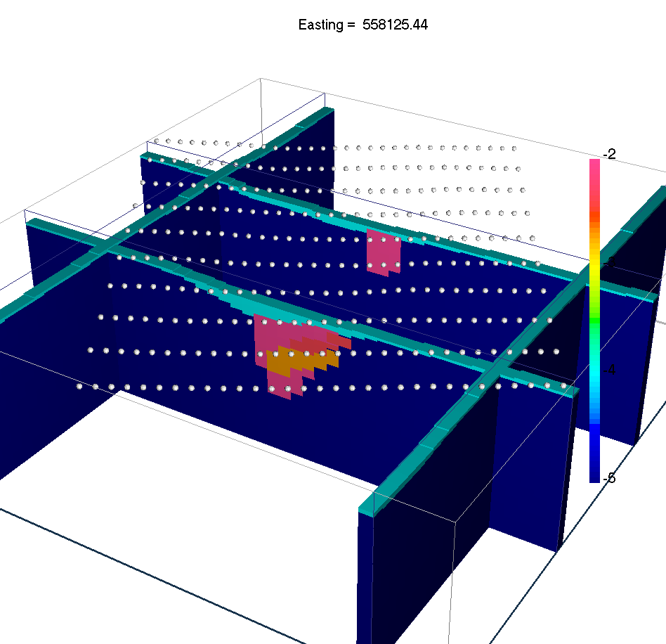
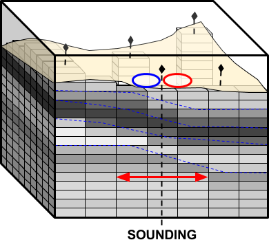
Sections through the true 3D conductivity model