9.1.1. Processing Gravity Data

Here, we show how GIFtools can be used to carry out processing steps relevant to gravity data such as:

• Free-air correction

• Simple terrain correction

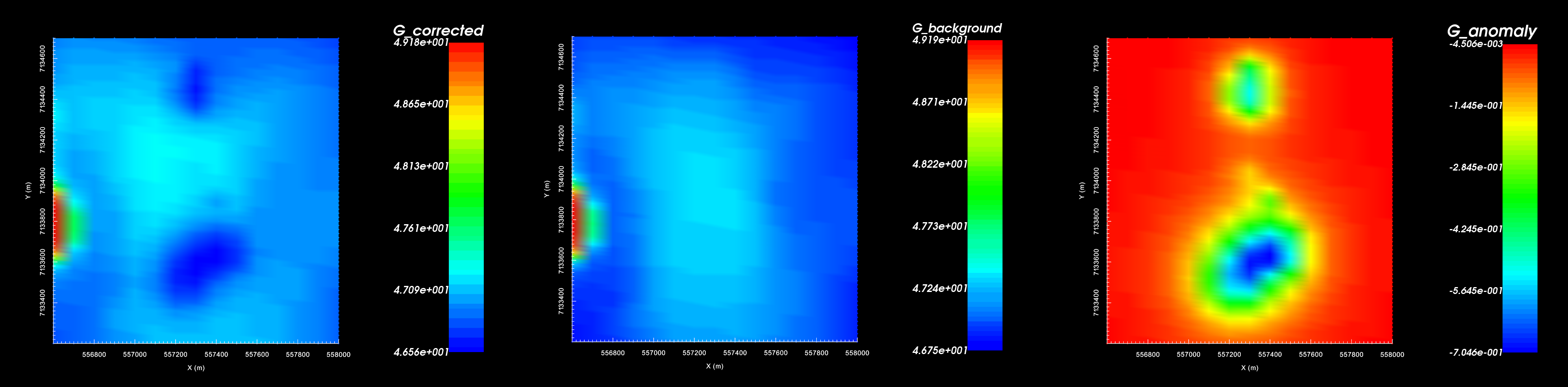
Gravity data after latitude and free-air correction (left). Background gravity (middle). Final gravity anomaly data (right).

9.1.1.1. Setup for the Processing Exercise

• Download the demo

• Open GIFtools

• Set the working directory

Tip

• Steps (without links) are also included with the download

• Requires at least GIFtools version 2.1.3 (Oct 2017) (login required)

9.1.1.2. Import files

In addition to raw geophysical data, you may have access to topographical information. If this information is available to you, it can be imported into GIFtools.

• Import the topography data (3D GIF format)

• Import raw gravity data (GIF format with data in mGal)

Tip

• Use Edit → Rename to change what objects in GIFtools are called

• For any data object, edit the data headers. We set the raw gravity data to “G_raw”

• Raw data were generated synthetically using the best-available density model for TKC and “un-processing” the data.

9.1.1.3. Latitude and Free-Air Correction

Generally, this processing step has been done by the client. However to demonstrate some basic functionality within GIFtools, we will perform simple latitude (\(g_l\)) and free-air (\(g_{fa}\)) corrections on the raw gravity data (\(g_{raw}\)) such that.

\[g_{corr} = g_{raw} - g_l + g_{fa} \;.\]

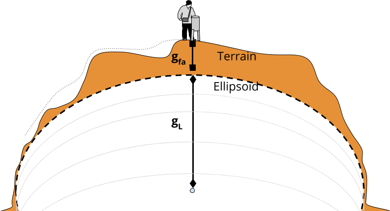
The latitude correction accounts for all of the mass contained within the reference ellipsoid approximation of the Earth. Generally a distinct latitude correction is applied for every survey location. However we will only be applying a constant value correction to the data; wherein we assume all survey locations are at a latitude of 64 \(\! ^o\) N.

The latitude correction (Int’l grav. formula 1967) in mGal is given by

\[\begin{split}\begin{align} \Delta g_l &= 978 \, 031.8 \times \big [ 1 + 0.0053024 \, sin^2 \phi - 0.0000059 \, sin^2 (2\phi) \big ] \\ &= 982217.559014 \textrm{ mGal at TKC} \end{align}\end{split}\]

The free-air correction accounts for the fact that the latitude correction is weaker the further you are from the Earth. GIFtools will be used to apply a specific free-air correction to each observation. The following expressions can be use to compute the latitude and free-air corrections. The free air correction: in mGal is given by:

\[\Delta g_{fa} = 0.3086 \times Elevation(m)\]

To apply these corrections to the raw data, carry out the following steps using the constant calculator:

• With the latitude correction provided (982217.559014 mGal) remove this value from the raw data and create a new column. Carry all decimal places!

• Compute the free-air correction that must be added to each survey location.

• Apply the free-air correction.

Tip

To keep track of data columns, remember to edit data headers.

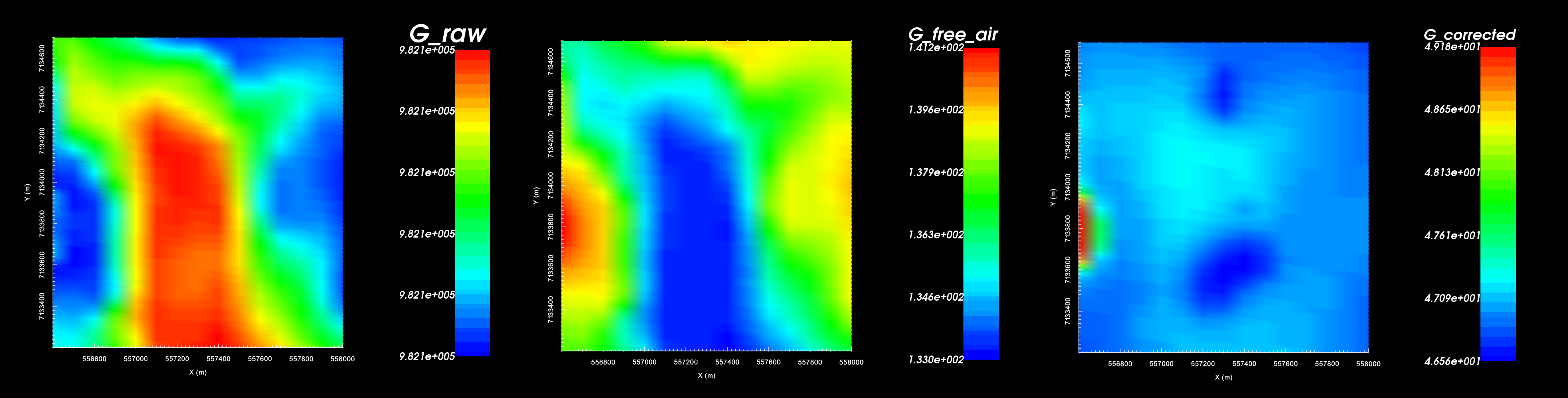
Raw gravity data (left). Free-air correction based on elevation (middle). Gravity data after latitude and free-air correction (right).

9.1.1.4. Topography and Regional Geology Correction

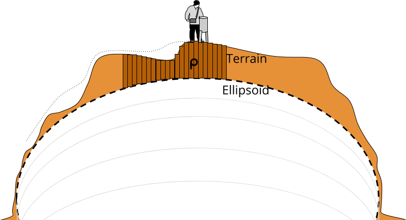
At this point, we have accounted for all gravity contributions from matter that lies below a surface elevation of 0 m; e.g. the latitude and free-air corrections. We must now remove the background gravity contribution from all regional mass that lies above 0 m elevation. If the topography is flat, you may choose to use a slab correction. Here, we show how GIFtools can remove the background contribution while taking into account the regional topography.

9.1.1.4.1. Create a Mesh

Here, we create a mesh which defines the regional geology. The mesh should extend vertically downward to an elevation of 0 m. We do not want to pad below this depth because we have already accounted for the mass lying below 0 m. The mesh should extend as far as possible horizontally so that gravity contributions outside the survey area are accounted for.

• Create a mesh using gravity data with the following parameters:

  • Don’t forget to apply topography when creating the mesh!

  • Core cell widths = 25 m

  • Extent above = 0 m

  • Depth of investigation = 425 m

  • Padding = 2000 m on each side, 0 m in depth

  • Padding factor = 1.2

Tip

Here, the mesh does not extend exactly to an elevation of 0 m. For the purposes of the exercise, this is fine. In practice however, it would be wise to extend the mesh to exactly 0 m because you have accounted for all mass below that elevation already.

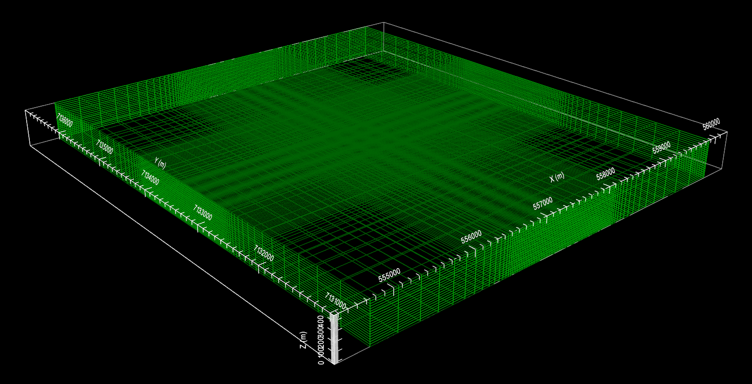
Mesh for use in background gravity removal.

9.1.1.4.2. Create Active Cells from Topography

Here, we account for the local topography. Since air cells contribute negligibly towards the observe data, we do not need to include them when modeling the background gravity.

• Using your gravity data, create an active cells model from topography. Choose ‘from tops of cells’

9.1.1.4.3. Create a Constant Density Model

At TKC, we know that the kimberlite pipes are within a granitoid host. We will assume a background density of 2.7 g/cc and create a background physical property model.

• Using the active cells model, create a constant geological model

• Assign a value of 2.7 g/cc for the background cells through edit geology definitions. You may also want to set I/0 headers and/or rename headers

• Create a physical property model (GIF model) from the geological model

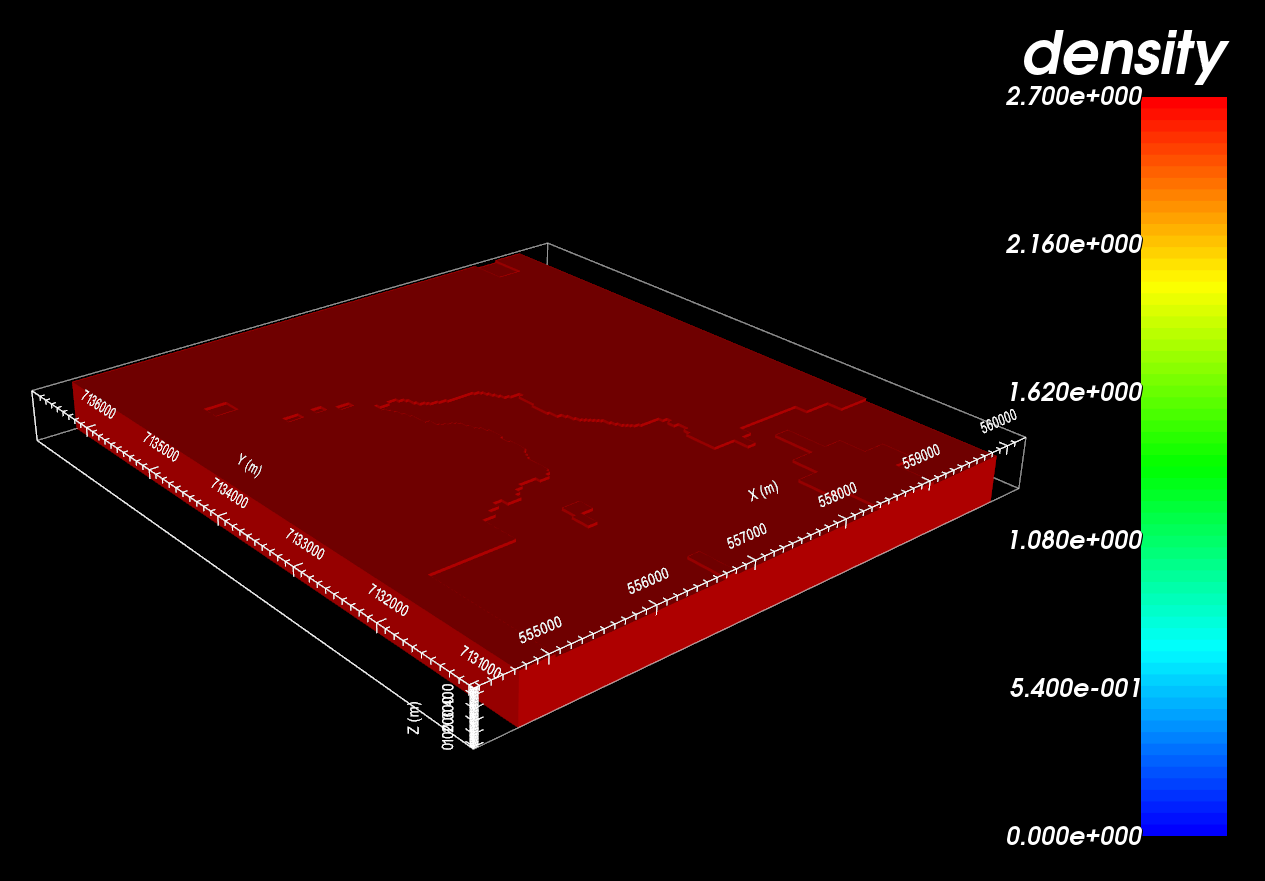
Constant density model for removing background gravity.

9.1.1.4.4. Predict Background Gravity and Load to GIFtools

We now have all the items necessary to forward model the background gravity contribution.

• Create Grav3D forward model through create forward modeling

• Select the forward modeling object and edit options to link

  • GIF Model

  • Data locations

  • Topography

• Write files

• Run GZFOR3D

• Load predicted data

9.1.1.4.5. Remove the Background Gravity

To remove the background gravity from your data:

• Use add data from another GRAVdata object to add the background gravity to the gravity data object where you are doing your processing

• Use the Calculator to subtract the background data; which should result in just the gravity anomaly remaining

Gravity data after latitude and free-air correction (left). Background gravity (middle). Final gravity anomaly data (right).