Here, we show how GIFtools can be used to invert gravity anomaly data. We consider the case where we have a set of field observations and some a priori knowledge of the local geology; for this example, we know the anomaly is produced by the TKC kimberlites. We assume that all necessary corrections have been applied to the raw gravity data; see the processing gravity data exercise. The goal of this exercise is to invert the gravity anomaly data to recover the optimum density model. Several inversion will be run to show the impact of reference models and various penalty terms on the final inversion result.
Tip
The same workflow can be used to invert magnetic data for an arbitrary susceptibility or magnetic vector model.
Steps (without links) are also included with the download
Requires at least GIFtoolsversion2.1.3(Oct2017) (login required)
9.1.3.3. Assign Uncertainties and Set I/O Headers
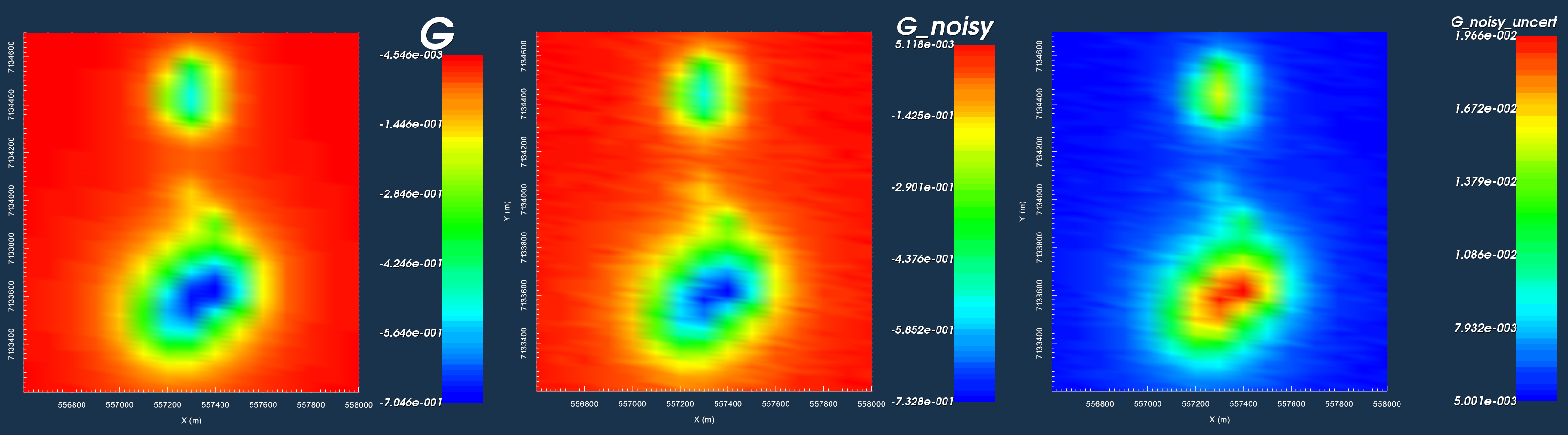
Assigning appropriate uncertainties to the data is necessary for running stable and successful inversions with GIFtools. Because the observed gravity data were generated synthetically, we will add random noise before assigning the uncertainties. Because the statistics of the noise are known, they can be used to assign the correct uncertainties. Complete the following steps:
Here, we perform the most basic type of gravity anomaly inversion. No a priori information is used in the inversion. Default inversion parameters use least-squares penalties on the model and its gradients. As a result, we expect the inversion to recover a smooth model. To run the inversion and view results:
Sensitivity Tab: set mesh, observed data and topography
Inversion Tab:
Set the active cells
Note
As a general best practice, in the absence of a priori
information, \(\alpha\) values should be set such that all
components of the regularization have equal weight. Based
on the core mesh discretization used in this problem:
\(\alpha_s = \left[\frac{1}{dx}\right]^2 = 0.0016\),
\(\alpha_x=\alpha_y=\alpha_z = 1\)
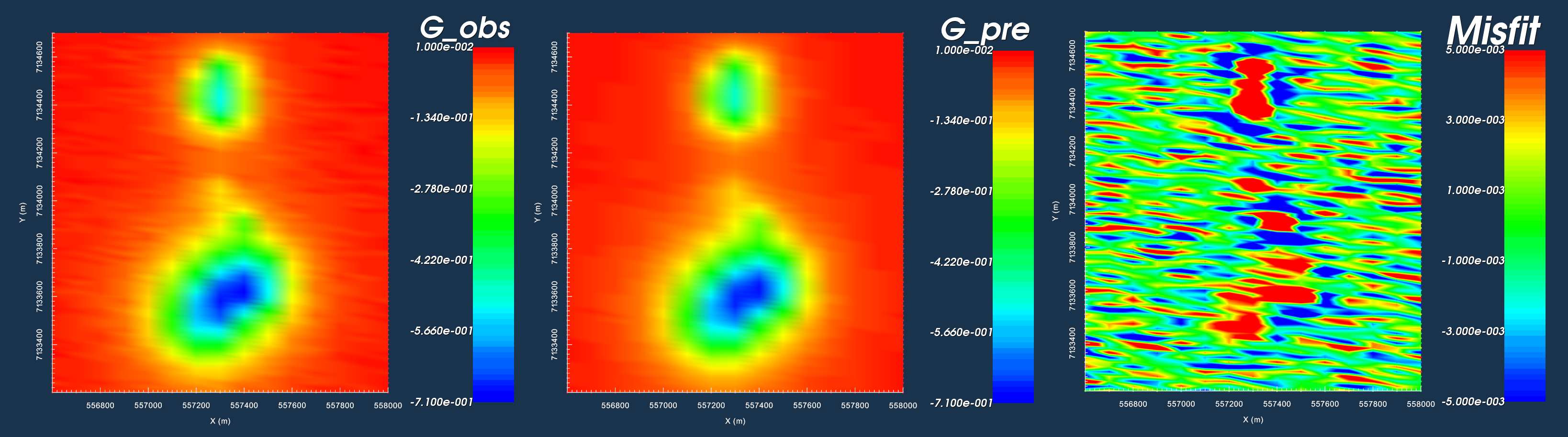
Generally, the data predicted using the recovered model matches the shape and character of the observed anomalies
However, large misfits are clustered around the locations of recovered structures
The general distribution of density contrasts is recovered through inversion
By using the default set of inversion parameters however, we recovered a very smooth density contrast model
Because the inversion was set to recover a smooth model, the inversion placed positive density contrast values (red) around the outside of the recovered structures
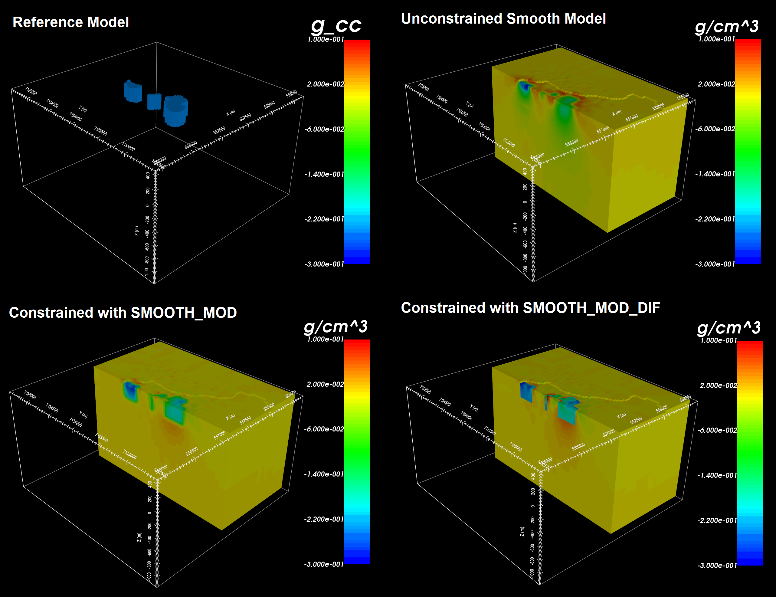
Here, we show the impact of reference models on the final inversion result.
Two inversion will be run - one using SMOOTH_MOD and
one using SMOOTH_MOD_DIFF. Both inversions are
constrained with the model that was made using the geological surface map (see
here). To complete this exercise:
Examine the differences in recovered models using SMOOTH_MOD and SMOOTH_MOD_DIF
Examine the differences in data misfit for data predicted using SMOOTH_MOD and SMOOTH_MOD_DIF inversions
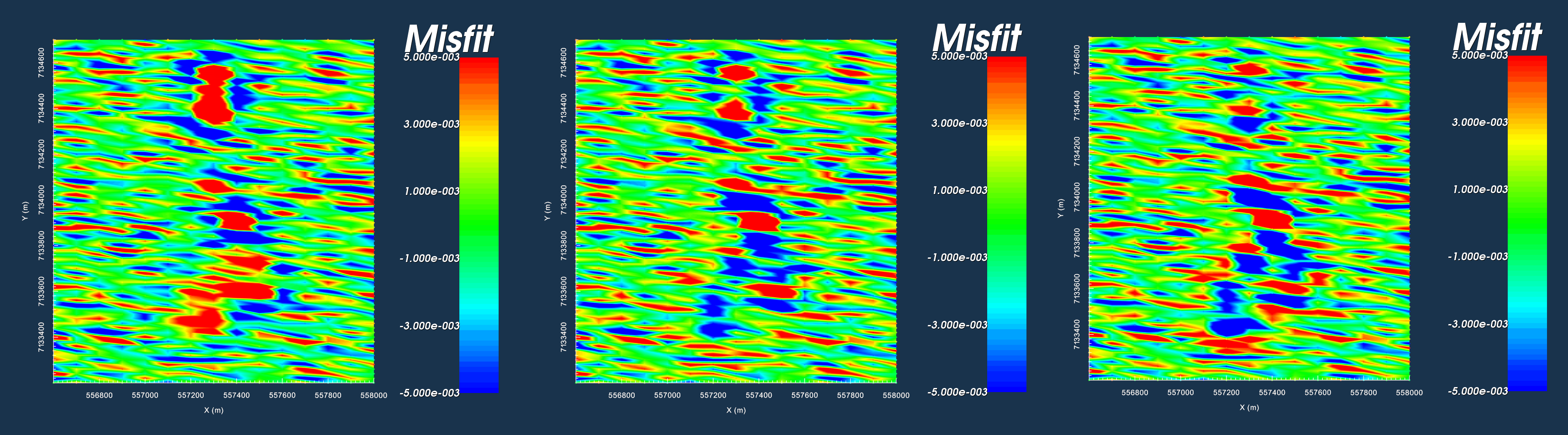
Data misfit thresholded at +/- 0.005 for the unconstrained smooth model (left), SMOOTH_MOD (middle) and SMOOTH_MOD_DIF (right).
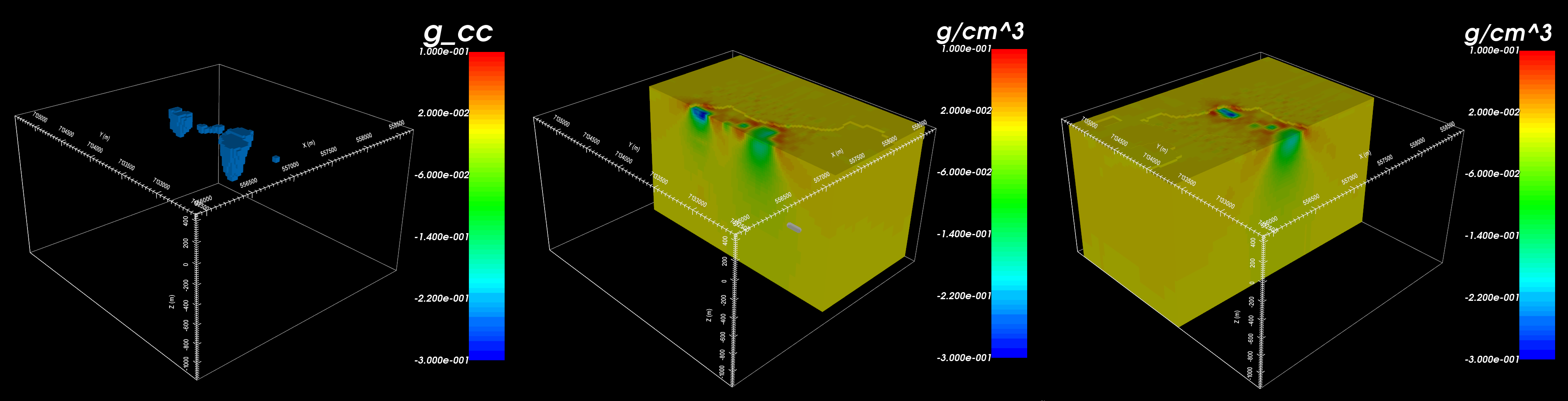
Reference model from geological unit image (top-left). Model recovered using unconstrained smooth inversion (top-right). Model recovered using SMOOTH_MOD (bottom-left). Model recovered using SMOOTH_MOD_DIF (bottom-right).
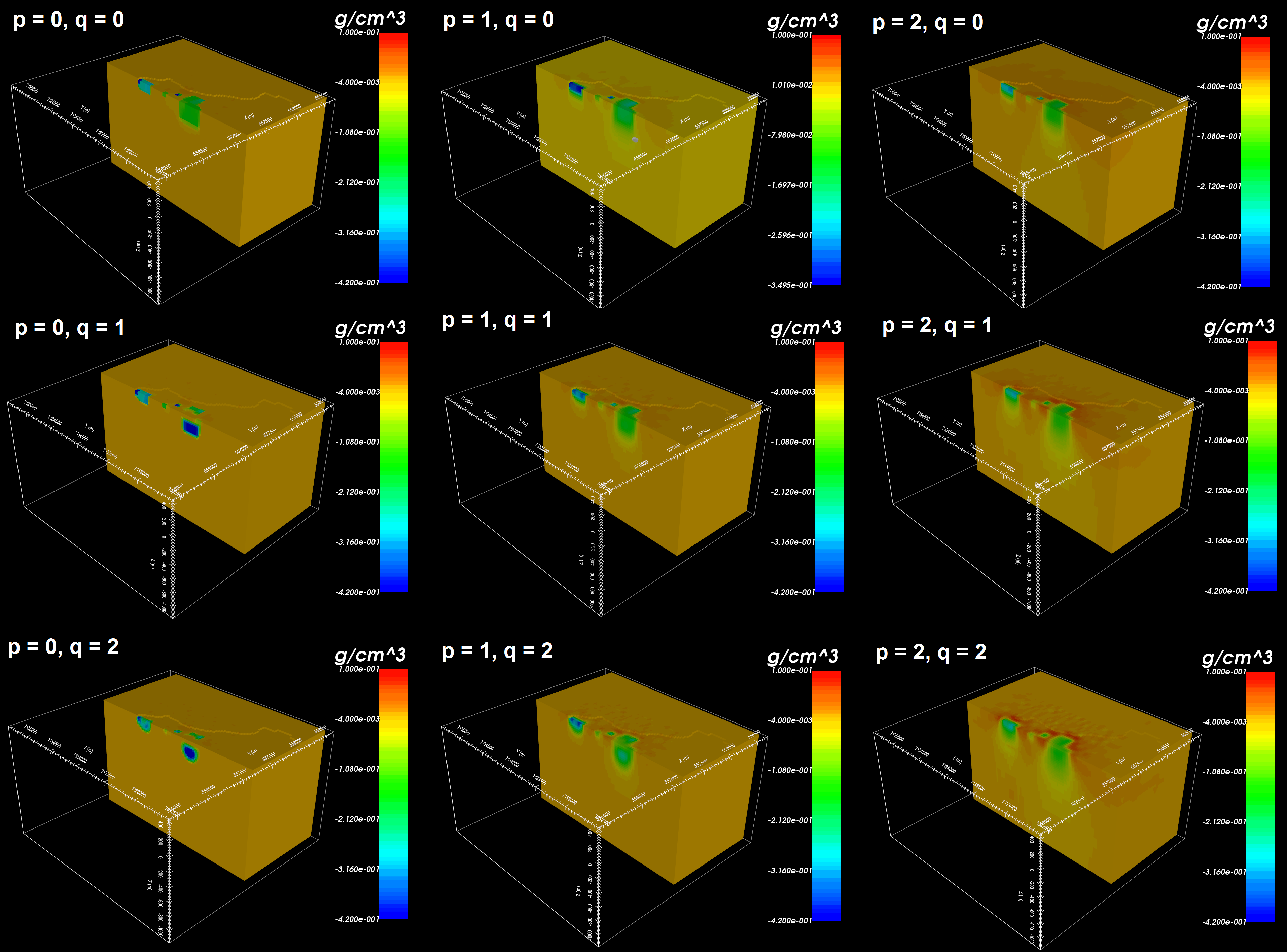
Here, we show how compact and blocky models can be recovered by changing certain inversion parameters. Smooth models are recovered when the compactness parameter (p) and the set of blockiness parameters (q) are set to a value of 2. By decreasing the compactness parameter value, we recover models that have a smaller number of non-zero values; that is, models which fit the observed data using more compact structures. By decreasing the blockiness parameter value, we recover models that have a smaller number of non-zero gradients; that is, models which fit the observed data using structures that have very sharp edges. To complete this exercise: