9.1.2. Forward Modeling and Hypothesis Testing
Here, we simulate synthetic data based on a surface geology map and compare it to the observed gravity data. A reasonable match ensures that our current geological understanding is able to explain the cause of the anomaly.
Tip
The same workflow can be used to predict magnetic data for an arbitrary susceptibility or magnetic vector model.
A synthetic density model (left). Predicted data from the model (middle). Difference between predicted and observed (right).
9.1.2.1. Setup for the Forward Modeling Exercise
If you have completed the tutorial “Processing Gravity Data”:
Open your final GIFtools project
Set the working directory (if you want to change it)
If you have NOT completed the previous tutorial, you must complete the following steps:
Open GIFtools
Tip
Steps (without links) are also included with the download
Requires at least
GIFtools version 2.1.3 (Oct 2017)(login required)
9.1.2.2. Import files
In addition to geophysical data, you may have access to topographical information and/or geological surface maps/cross-sections. If this information is available to you, it can be imported to GIFtools. Here, we have surface topography and files which define several geological units through surface mapping.
Import the topography data (3D GIF format). This was imported in the previous exercise
Import field observed gravity anomaly data (GIF format with data in mGal). This was the final result of the previous exercise
Import the geology image and link to topography (Image is plane view)
Tip
Use Edit → Rename to change what objects in GIFtools are called
For any data object, edit the data headers. We set the gravity anomaly data to “Gravity (mGal)”
Observed gravity anomaly data were generated synthetically using the best-available density model for TKC.
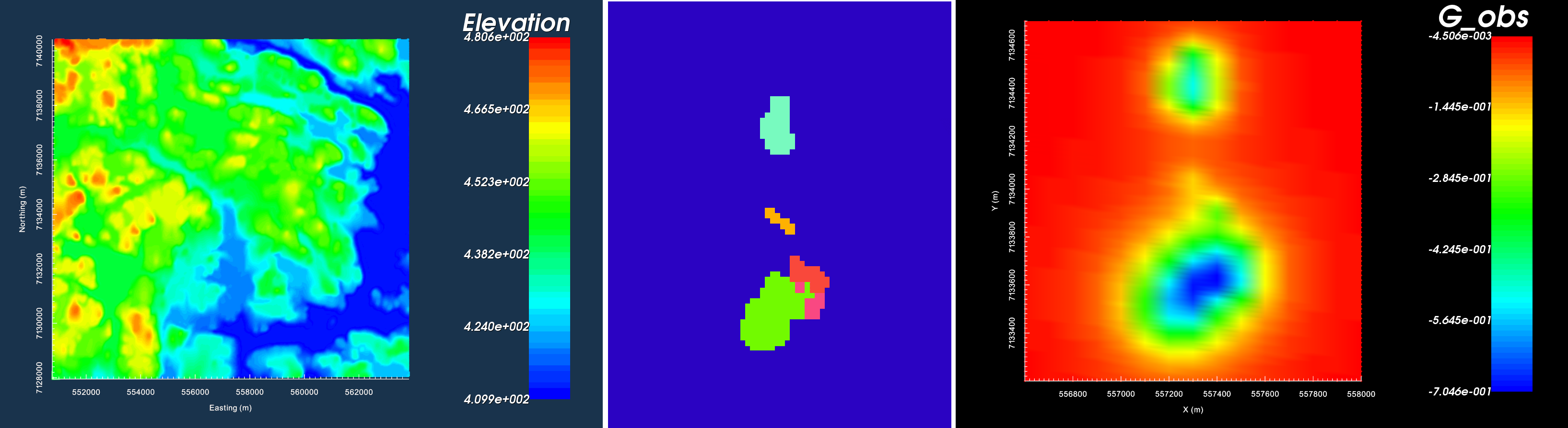
Topography imaged in VTK (left). Plan-view image for surface geological mapping (middle). Gravity anomaly data in mGal (right).
9.1.2.3. Create a Survey
Ultimately, we would like to predict gravity anomaly data for a model of our choosing and compare it against a set of field observations. To accomplish this, we must first create a survey; which has the same properties as the actual survey that was performed. To create the survey, there are two approaches:
9.1.2.3.1. Approach 1: Survey at exact locations
Using this approach, we will be able to predict gravity data at the EXACT same locations as the field observations. Later on, this will allow us to compute the difference between the predicted and observed data. Steps are as follows:
Make a copy of the gravity data
Through Set I/O headers, remove the I/O header for gravity anomaly data column by setting it to blank
Delete the data columns for any preexisting gravity data (data cannot be deleted if it has an assigned I/O header)
9.1.2.3.2. Approach 2: Custom locations
- Create simple survey
Set the survey type as ‘Gravity’
Link the survey to the known topography at TKC
Set the height above topography to 10 m
- Set the following parameters:
Easting origin = 556,600
Northing origin = 7,133,200
Bearing = 0
Line length = 1,500
Number of survey lines = 15
Data spacing = 20
Line spacing = 100
Tip
Since the survey parameters are exactly known, approach 1 and approach 2 produce the same thing.
Both the observed gravity and survey are ‘gravity data’ objects. Thus they have the same properties and undergo identical actions.
Edit data headers was used to make the colourbar titles the same in the plot below.
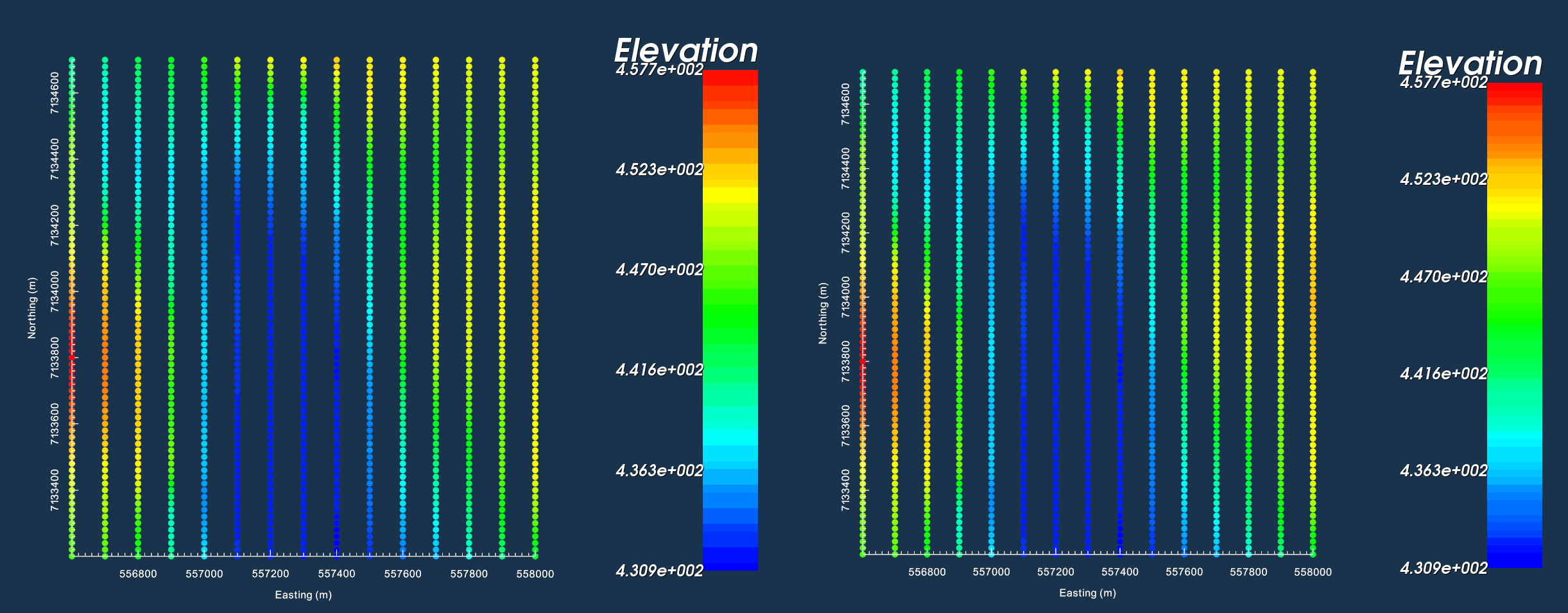
Data location from observed data file (left). Data locations for synthetic survey (right).
9.1.2.4. Create Mesh from Gravity Survey
To predict field data, we must define the domain by creating a mesh. GIFtools can create meshes based on the data locations and the local topography.
- Create mesh from gravity data
Don’t forget to apply topography when creating the mesh!
Core cell widths = 25 m
Extent above = 0 m
Depth of investigation = 400 m
Padding = 500 m on each side, 1000 m in depth
Padding factor = 1.2
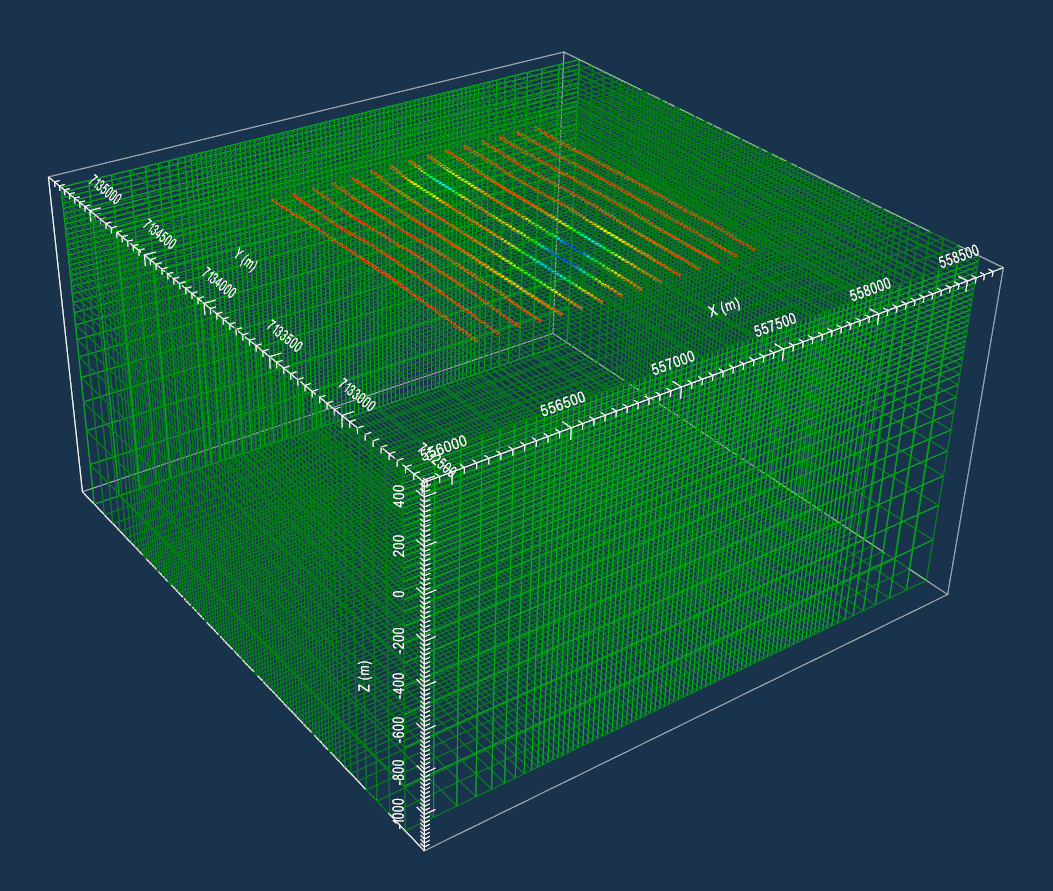
Mesh created from survey and viewed in VTK. Gravity anomaly data from the survey have been imported at their locations.
Tip
There are other ways to make meshes. If available, you could import a pre-existing mesh or create and OcTree mesh.
9.1.2.5. Create Models
In this step, we design a density model for the geological structure we think will explain the data. We will show that test models can be made quickly using a priori geological information, as opposed to creating a model comprised of uniform blocks. At TKC, we know:
The surface topography
The gravity anomaly is likely caused by the presence of kimberlite pipes
The surface distribution of geological units obtained from geological mapping
The approximate density of kimberlites relative to the host
However, we don’t know:
How far down the kimberlites extend
The thickness of any of the kimberlite pipes as a function of depth
The thickness of the overlying till
9.1.2.5.1. Create Active Cells Model from Topography
Regions above the topography have an effective density of 0 and do not contribute towards the gravitational pull experienced at observation locations. For potential field problems, we MUST ensure that data locations lie outside the region of active cells (e.g. within the air cells). Here, we will use the topography data to create an active cells model.
Creating active cell model from topography. Choose ‘from tops of cells’
9.1.2.5.2. Create Density Model through Model Builder
Now that we have topography, a mesh, and an active cells model, we can create a geological model. To approximate pipe-like structures, we will use the horizontal distributions of each geological unit (obtained from the plan-view image), and project these units down to a desired depth. We will then assign density contrast values to all geological units. Once the geological model has been created, we will output a physical property model which can be used in the forward model. To accomplish this, apply the following steps:
Create geology model from plan-view image (Use a thickness of 200 m)
Set physical propert values for units in the newly created GEO model (The approximate density contrast values for the kimberlites and till relative to the host is found here). Units should be g/cc. You may also want to set I/0 headers and/or rename headers
Create GIF model from the physical properties in the GEO model
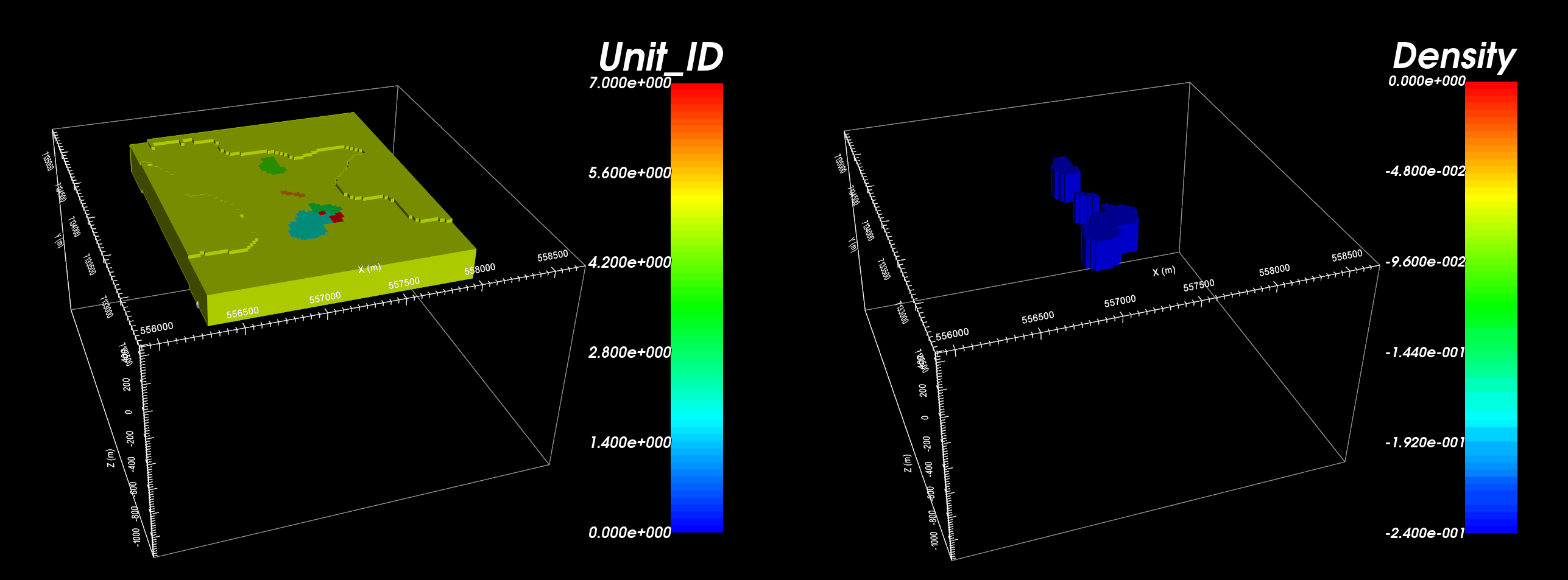
Geological model created with each colour representing a different units (left). Density contrast in g/cc relative to host (right).
9.1.2.6. Forward Model the Data
We now have all the objects we need to create the files for the forward model and run the fortran code. This is accomplished by carrying out the following steps:
Create Grav3D forward model through create forward modeling
- Select the forward modeling object and edit options to link
GIF Model
Data locations
Topography
9.1.2.7. Load Predicted Data and Compare Against Observed Data
Here, we compare the observed data to the predicted data from our forward model. We will also show how the difference between both datasets can be computed and plotted.
Using add data from another object, add the observed data to the predicted gravity data
Using Calculator, subtract the predicted data from the observed data
View the data (observed, predicted and difference) from the final data object you created
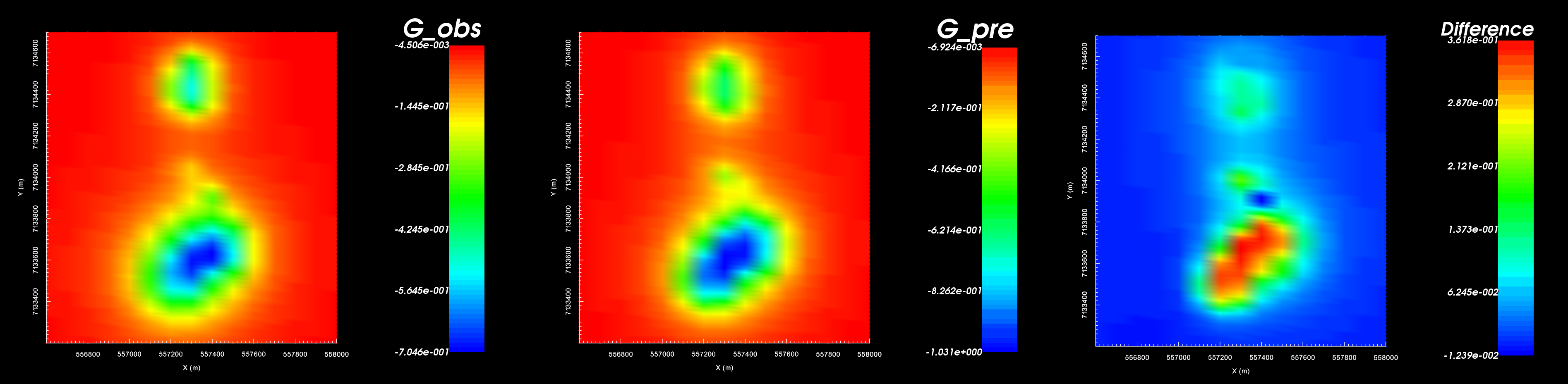
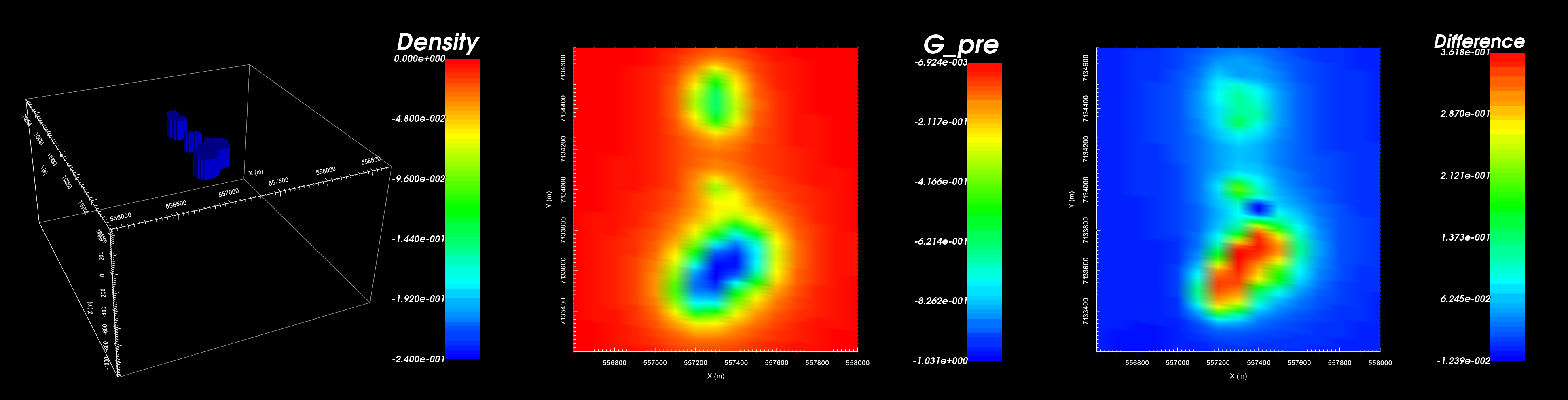
Observed data (left). Predicted data (middle). Observed - predicted (right).
Tip
Edit data headers to avoid confusion between predicted and observed data.
9.1.2.8. Results
Our synthetic model produces gravity anomalies of similar size and character.
The northern portion of the largest anomaly does not match between predicted and observed gravity data
The predicted data over-estimates the maximum anomaly amplitude
Our synthetic model explains the data, but the margins of various kimberlite facies and their density distributions remain unresolved.